1. Worst-Case Execution Time and Energy Analysis

1.1 Introduction

Timing predictability is extremely important for hard real-time embedded systems employed in application domains such as automotive electronics and avionics. Schedulability analysis techniques can guarantee the satisfiability of timing constraints for systems consisting of multiple concurrent tasks. One of the key inputs required for the schedulability analysis is the worst-case execution time (WCET) of each of the tasks. WCET of a task on a target processor is defined as its maximum execution time across all possible inputs.

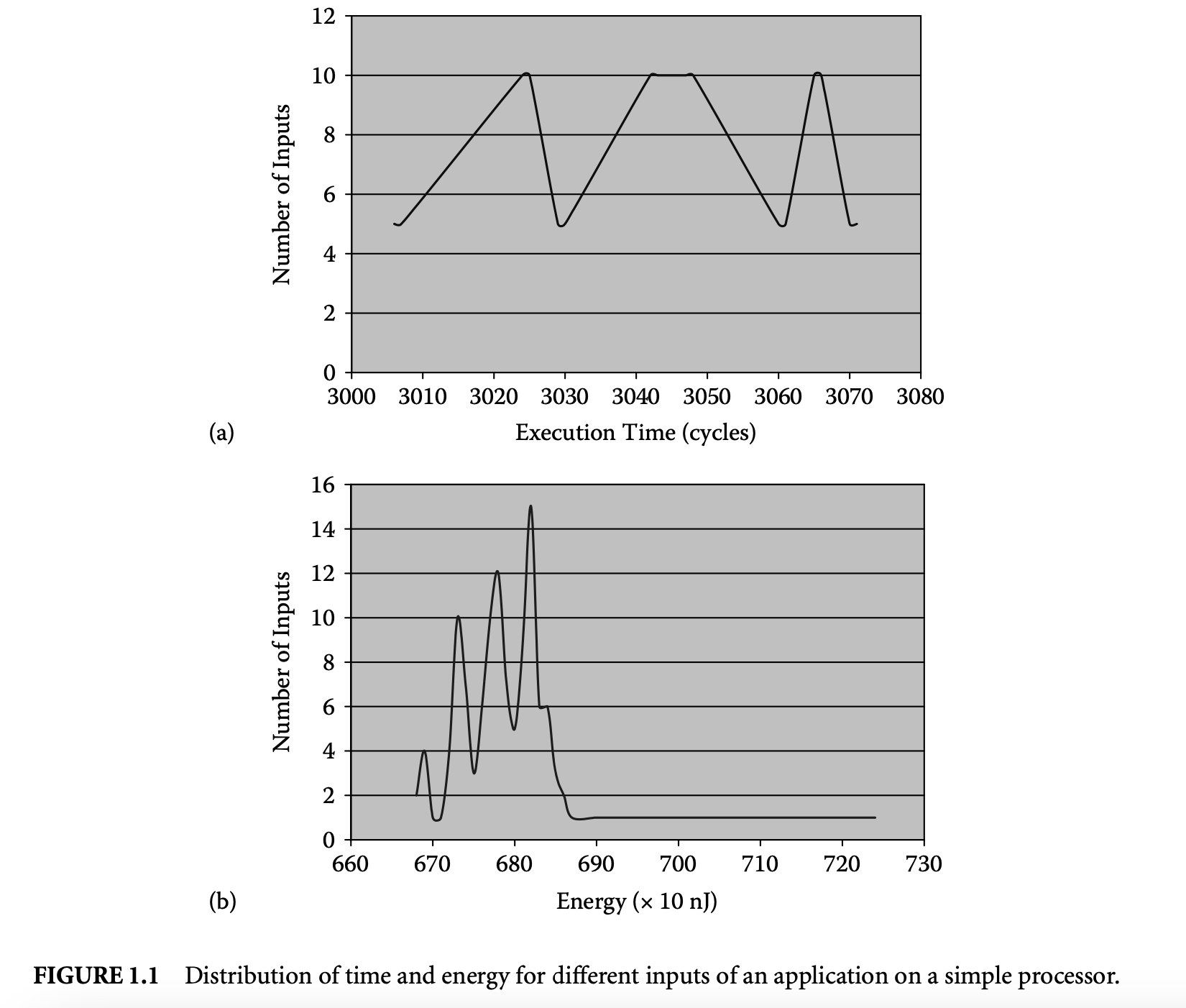
Figure 1.1a and Figure 1.2a show the variation in execution time of a $quicksort$ program on a simple and complex processor, respectively. The program sorts a five-element array. The figures show the distribution of execution time (in processor cycles) for all possible permutations of the array elements as inputs. The maximum execution time across all the inputs is the WCET of the program. This simple example illustrates the inherent difficulty of finding the WCET value:

• Clearly, executing the program for all possible inputs so as to bound its WCET is not feasible. The problem would be trivial if the worst-case input of a program is known a priori. Unfortunately, for most programs the worst-case input is unknown and cannot be derived easily.

• Second, the complexity of current micro-architectures implies that the WCET is heavily influenced by the target processor. This is evident from comparing Figure 1.1a with Figure 1.2a. Therefore, the timing effects of micro-architectural components have to be accurately accounted for.

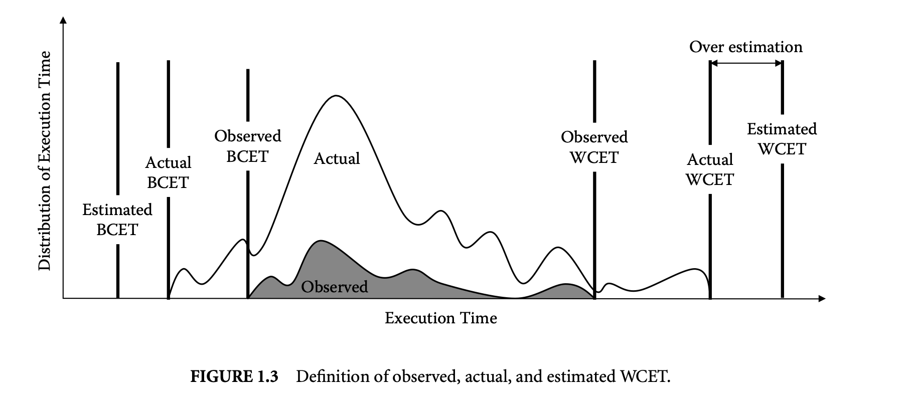
Static analysis methods estimate a bound on the WCET. These analysis techniques are conservative in nature. That is, when in doubt, the analysis assumes the worst-case behavior to guarantee the safety of the estimated value. This may lead to overestimation in some cases. Thus, the goal of static analysis methods is to estimate a safe and tight WCET value. Figure 1.3 explains the notion of safety and tightness in the context of static WCET analysis. The figure shows the variation in execution time of a task. The actual WCET is the maximum possible execution time of the program. The static analysis method generates the estimated WCET value such that estimated WCET$\ge$actual WCET. The difference between the estimated and the actual WCET is the overestimation and determines how tight the estimation is. Note that the static analysis methods guarantee that the estimated WCET value can never be less than the actual WCET value. Of course, for a complex task running on a complex processor, the actual WCET value is unknown. Instead, simulation or execution of the program with a subset of possible inputs generates the observed WCET, where observed WCET$\le$actual WCET. In other words, the observed WCET value is not safe, in the sense that it cannot be used to provide absolute timing guarantees for safety-critical systems. A notion related to WCET is the BCET (best-case execution time), which represents the minimum execution time across all possible inputs. In this chapter, we will focus on static analysis techniques to estimate the WCET. However, the same analysis methods can be easily extended to estimate the BCET.

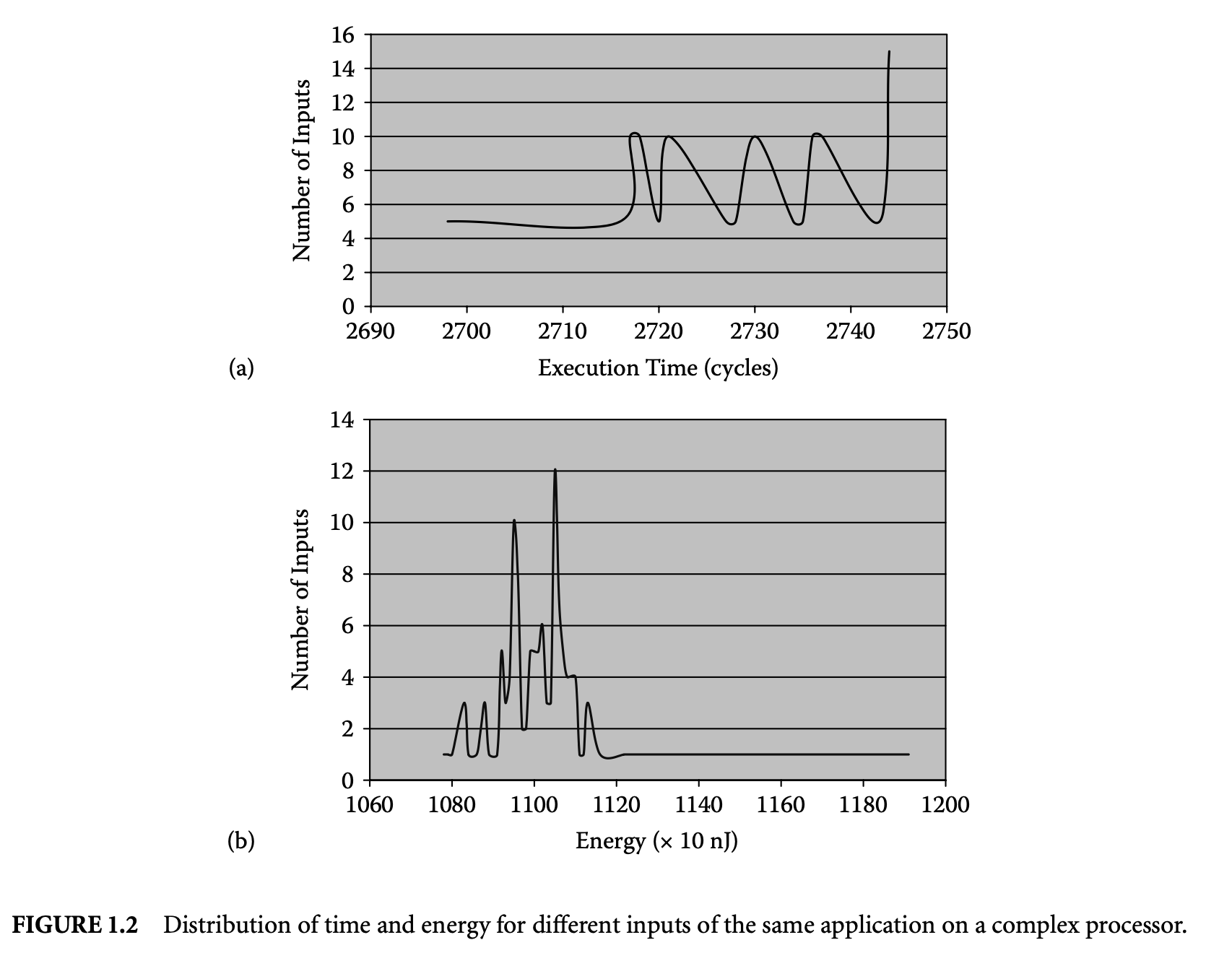
Apart from timing, the proliferation of battery-operated embedded devices has made energy consumption one of the key design constraints. Increasingly, mobile devices are demanding improved functionality and higher performance. Unfortunately, the evolution of battery technology has not been able to keep up with performance requirements. Therefore, designers of mission-critical systems, operating on limited battery life, have to ensure that both the timing and the energy constraints are satisfied under all possible scenarios. The battery should never drain out before a task completes its execution. This concern leads to the related problem of estimating the worst-case energy consumption of a task running on a processor for all possible inputs. Unlike WCET, estimating the worst-case energy remains largely unexplored even though it is considered highly important [86], especially for mobile devices. Figure 1.1b and Figure 1.2b show the variation in energy consumption of the quick sort program on a simple and complex processor, respectively.

A natural question that may arise is the possibility of using the WCET path to compute a bound on the worst-case energy consumption. As energy = average power $\times$ execution time, this may seem like a viable solution and one that can exploit the extensive research in WCET analysis in a direct fashion. Unfortunately, the path corresponding to the WCET may not coincide with the path consuming maximum energy. This is made apparent by comparing the distribution of execution time and energy for the same program and processor pair as shown in Figure 1.1 and Figure 1.2. There are a large number of input pairs $⟨I_1,I_2⟩$ in this program, where $time(I_1)<time(I_2)$, but $energy(I_1)>energy(I_2)$. This happens as the energy consumed because of the switching activity in the circuit need not necessarily have a correlation with the execution time. Thus, the input that leads to WCET may not be identical to the input that leads to the worst-case energy.

The execution time or energy is affected by the path taken through the program and the underlying micro-architecture. Consequently, static analysis for worst-case execution time or energy typically consists of three phases. The first phase is the program path analysis to identify loop bounds and infeasible flows through the program. The second phase is the architectural modeling to determine the effect of pipeline, cache, branch prediction, and other components on the execution time (energy). The last phase, estimation, finds an upper bound on the execution time (energy) of the program given the results of the flow analysis and the architectural modeling.

Recently, there has been some work on measurement-based timing analysis[92, 6, 17]. This line of work is mainly targeted toward soft real-time systems, such as multimedia applications, that can afford to miss the deadline once in a while. In other words, these application domains do not require absolute timing guarantees. Measurement-based timing analysis methods execute or simulate the program on the target processor for a subset of all possible inputs. They derive the maximum observed execution time (see the definition in Figure 1.3) or the distribution of execution time from these measurements. Measurement-based performance analysis is quite useful for soft real-time applications, but they may underestimate the WCET, which is not acceptable in the context of safety-critical, hard real-time applications. In this article, we only focus on static analysis techniques that provide safe bounds on WCET and worst-case energy. The analysis methods assume uninterrupted program execution on a single processor. Furthermore, the program being analyzed should be free from unbounded loops, unbounded recursion, and dynamic function calls [67].

The rest of the chapter is organized as follows. We proceed with programming-language-level WCET analysis in the next section. This is followed by micro-architectural modeling in Section 1.3. We present a static analysis technique to estimate worst-case energy bound in Section 1.4. A brief description of existing WCET analysis tools appears in Section 1.5, followed by conclusions.

1.2 Programming-Language-Level WCET Analysis

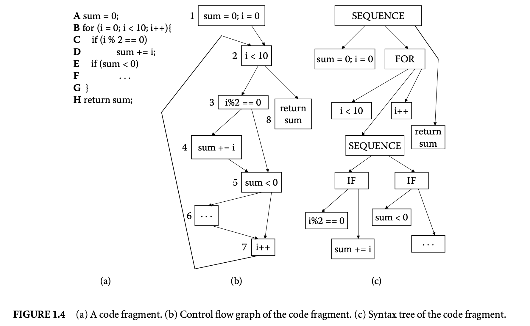
We now proceed to discuss static analysis methods for estimating the WCET of a program. For WCET analysis of a program, the first issue that needs to be determined is the program representation on which the analysis will work. Earlier works [73] have used the syntax tree where the (nonleaf) nodes correspond to programming-language-level control structures. The leaves correspond to basic blocks -- maximal fragments of code that do not involve any control transfer. Subsequently, almost all work on WCET analysis has used the control flow graph. The nodes of a control flow graph (CFG) correspond to basic blocks, and the edges correspond to control transfer between basic blocks. When we construct the CFG of a program, a separate copy of the CFG of a function $f$ is created for every distinct call site of $f$ in the program such that each call transfers control to its corresponding copy of CFG. This is how interprocedural analysis will be handled. Figure 4 shows a small code fragment as well as its syntax tree and control flow graph representations.

One important issue needs to be clarified in this regard. The control flow graph of a program can be either at the source code level or at the assembly code level. The difference between the two comes from the compiler optimizations. Our program-level analysis needs to be hooked up with micro-architectural modeling, which accurately estimates the execution time of each instruction while considering the timing effects of underlying microarchitectural features. Hence we always consider the assembly-code-level CFG. However, while showing our examples, we will show CFG at the source code level for ease of exposition.

1.2.1 WCET Calculation

We explain WCET analysis methods in a top-down fashion. Consequently, at the very beginning, we present WCET calculation -- how to combine the execution time estimates of program fragments to get the execution time estimate of a program. We assume that the loop bounds (i.e., the maximum number of iterations for a loop) are known for every program loop; in Section 2 we outline some methods to estimate loop bounds.

In the following, we outline the three main categories of WCET calculation methods. The path-based and integer linear programming methods operate on the program's control flow graph, while the tree-based methods operate on the program's syntax tree.

1.2.1.1 Tree-Based Methods

One of the earliest works on software timing analysis was the work on timing schema[73]. The technique proceeds essentially by a bottom-up pass of the syntax tree. During the traversal, it associates an execution time estimate for each node of the tree. The execution time estimate for a node is obtained from the execution time estimates of its children, by applying the rules in the schema. The schema prescribes rules -- one for each control structure of the programming language. Thus, rules corresponding to a sequence of statements, if-then-else and while-loop constructs, can be described as follows.

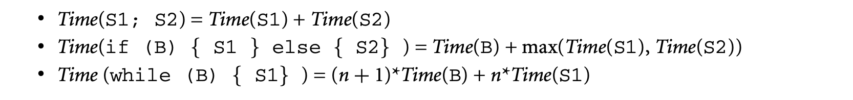
Here, $n$ is the loop bound. Clearly, S1, S2 can be complicated code fragments whose execution time estimates need to obtained by applying the schema rules for the control structures appearing in S1, S2. Extensions of the timing schema approach to consider micro-architectural modeling will be discussed in Section 1.3.5.

The biggest advantage of the timing schema approach is its simplicity. It provides an efficient compositional method for estimating the WCET of a program by combining the WCET of its constituent code fragments. Let us consider the following schematic code fragment $Pgm$. For simplicity of exposition, we will assume that all assignments and condition evaluations take one time unit.

i = 0; while (i<100) {if (B') S1 else S2; i++;}

If $\text{Time}(\text{S1})>\text{Time}(\text{S2})$, by using the rule for if-then-else statements in the timing schema we get

Now, applying the rule for while-loops in the timing schema, we get the following. The loop bound in this case is 100.

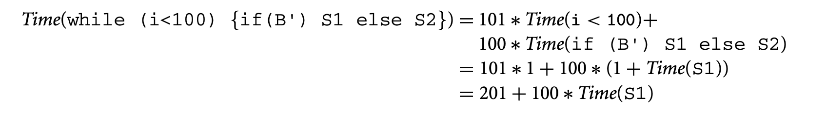
Finally, using the rule for sequential composition in the timing schema we get

The above derivation shows the working of the timing schema. It also exposes one of its major weaknesses. In the timing schema, the timing rules for a program statement are local to the statement; they do not consider the context with which the statement is arrived at. Thus, in the preceding we estimated the maximum execution time of if (B') S1 else S2 by taking the execution time for evaluating B and the time for executing S1 (since time for executing S1 is greater than the time for executing S2). As a result, since the if-then-else statement was inside a loop, our maximum execution time estimate for the loop considered the situation where S1 is executed in every loop iteration (i.e., the condition B' is evaluated to true in every loop iteration).

However, in reality S1 may be executed in very few loop iterations for any input; if Time(S1) is significantly greater than Time(S2), the result returned by timing schema will be a gross overestimate. More importantly, it is difficult to extend or augment the timing schema approach so that it can return tighter estimates in such situations. In other words, even if the user can provide the information that "it is infeasible to execute S1 in every loop iteration of the preceding program fragment $Pgm$," it is difficult to exploit such information in the timing schema approach. Difficulty in exploiting infeasible program flows information (for returning tighter WCET estimates) remains one of the major weaknesses of the timing schema. We will revisit this issue in Section 1.2.2.

1.2.1.2 Path-Based Methods

The path-based methods perform WCET calculation of a program $P$ via a longest-path search over the control flow graph of $P$. The loop bounds are used to prevent unbounded unrolling of the loops. The biggest disadvantage of this method is its complexity, as in the worst-case it may amount to enumeration of all program paths that respect the loop bounds. The advantage comes from its ability to handle various kinds of flow information; hence, infeasible path information can be easily integrated with path-based WCET calculation methods.

One approach for restricting the complexity of longest-path searches is to perform symbolic state exploration (as opposed to an explicit path search). Indeed, it is possible to cast the path-based searches for WCET calculation as a (symbolic) model checking problem [56]. However, because model checking is a verification method [13], it requires a temporal property to verify. Thus, to solve WCET analysis using model-checking-based verification, one needs to guess possible WCET estimates and verify that these estimates are indeed WCET estimates. This makes model-checking-based approaches difficult to use (see [94] for more discussion on this topic). The work of Schuele and Schneider [72] employs a symbolic exploration of the program's underlying transition system for finding the longest path, without resorting to checking of a temporal property. Moreover, they [72] observe that for finding the WCET there is no need to (even symbolically) maintain data variables that do not affect the program's control flow; these variables are identified via program slicing. This leads to overall complexity reduction of the longest-path search involved in WCET calculation.

A popular path-based WCET calculation approach is to employ an explicit longest-path search, but over a fragment of the control flow graph [31, 76, 79]. Many of these approaches operate on an acyclic fragment of the control flow graph. Path enumeration (often via a breadth-first search) is employed to find the longest path within the acyclic fragment. This could be achieved by a weighted longest-path algorithm (the weights being the execution times of the basic blocks) to find the longest sequence of basic blocks in the control flow graph for a program fragment. The longest-path algorithm can be obtained by a variation of Dijkstra's shortest-path algorithm [76]. The longest paths obtained in acyclic control flow graph fragments are then combined with the loop bounds to yield the program's WCET. The path-based approaches can readily exploit any known infeasible flow information. In these methods, the explicit path search is pruned whenever a known infeasible path pattern is encountered.

Integer Linear Programming (ILP)ILP combines the advantages of the tree and path-based approaches. It allows (limited) integration of infeasible path information while (often) being much less expensive than the path-based approaches. Many existing WCET tools such as aiT [1] and Chronos [44] employ ILP for WCET calculation.

The ILP approach operates on the program's control flow graph. Each basic block $B$ in the control flow graph is associated with an integer variable $N_B$, denoting the total execution count of basic block $B$. The program's WCET is then given by the (linear) objective function

where $\mathcal{B}$ is the set of basic blocks of the program, and $c_B$ is a constant denoting the WCET estimate of basic block $B$. The linear constraints on $N_B$ are developed from the flow equations based on the control flow graph. Thus, for basic block $B$,

where $E_{B^{\prime }\to B}$ ($E_{B\to B^{\prime }}$) is an ILP variable denoting the number of times control flows through the control flow graph edge $B^{\prime }\to B$ ($B\to B^{\prime \prime }$). Additional linear constraints are also provided to capture loop bounds and any known infeasible path information.

In the example of Figure 1.4, the control flow equations are given as follows. We use the numbering of the basic blocks $1$ to $8$ shown in Figure 1.4. Let us examine a few of the control flow equations. For basic block $1$, there are no incoming edges, but there is only one outgoing edge $1\to 2$. This accounts for the constraint $N_1=E_{1\to 2}$; that is, the number of executions of basic block $1$ is equal to the number of flowsfrom basic block 1 to basic block 2. In other words, whenever basic block 1 is executed, control flows from basic block 1 to basic block 2. Furthermore, since basic block 1 is the entry node, it is executed exactly once; this is captured by the constraint $N_1=1$. Now, let us look at the constraints for basic block 2; the inflows to this basic block are the edges $1\to 2$ and $7\to 2$ and the outflows are the edges $2\to 3$ and $2\to 8$. This means that whenever block 2 is executed, control must have flown in via either the edge $1\to 2$ or the edge $7\to 2$; this accounts for the constraint $E_{1\to 2}+E_{7\to 2}=N_2$. Furthermore, whenever block 2 is executed, control must flow out via the edge $2\to 3$ or the edge $2\to 8$. This accounts for the constraint $N_2=E_{2\to 3}+E_{2\to 8}$. The inflow/outflow constraints for the other basic blocks are obtained in a similar fashion. The full set of inflow/outflow constraints for Figure 4 are shown in the following.

The execution time of the program is given by the following linear function in $N_i$ variables ($c_i$ is a constant denoting the WCET of basic block $i$).

Now, if we ask the ILP solver to maximize this objective function subject to the inflow/outflow constraints, it will not succeed in producing a time bound for the program. This is because the only loop in the program has not been bounded. The loop bound information itself must be provided as linear constraints. In this case, since Figure 4 has only one loop, this accounts for the constraint

Using this loop bound, the ILP solver can produce a WCET bound for the program. Of course, the WCET bound can be tightened by providing additional linear constraints capturing infeasible path information; the flow constraints by default assume that all paths in the control flow graph are feasible. It is worthwhile to note that the ILP solver is capable of only utilizing the loop bound information and other infeasible path information that is provided to it as linear constraints. Inferring the loop bounds and various infeasible path patterns is a completely different problem that we will discuss next.

Before moving on to infeasible path detection, we note that tight execution time estimates for basic blocks (the constants $c_i$ appearing in the ILP objective function) are obtained by micro-architectural modeling techniques described in Section 3. Indeed, this is how the micro-architectural modeling and program path analysis hook up in most existing WCET estimation tools. The program path analysis is done by an ILP solver; infeasible path and loop bound information are integrated with the help of additional linear constraints. The objective function of the ILP contains the WCET estimates of basic blocks as constants. These estimates are provided by micro-architectural modeling, which considers cache, pipeline, and branch prediction behavior to tightly estimate the maximum possible execution time of a basic block $B$ (where $B$ is executed in any possible hardware state and/or control flow context).

1.2.2 Infeasible Path Detection and Exploitation

In the preceding, we have described WCET calculation methods without considering that certain sequences of program fragments may be infeasible, that is, not executed on any program input. Our WCET calculation methods only considered the loop bounds to determine a program's WCET estimate. In reality, the WCET calculation needs to consider (and exploit) other information about infeasible program paths. Moreover, the loop bounds also need to be estimated through an off-line analysis. Before proceeding further, we define the notion of an infeasible path.

Definition 1.1

Given a program $P$, let ${\mathcal{B}}_P$ be the set of basic blocks of $P$. Then, an infeasible path of $P$ is a sequence of basic blocks $\sigma$ over the alphabet ${\mathcal{B}}_P$, such that $\sigma$ does not appear in the execution trace corresponding to any input of $P$.

Clearly, knowledge of infeasible path patterns can tighten WCET estimates. This is simply because the longest path determined by our favorite WCET calculation method may be an infeasible one. Our goal is to efficiently detect and exploit infeasible path information for WCET analysis. The general problem of infeasible path detection is NP-complete [2]. Consequently, any approach toward infeasible path detection is an underapproximation -- any path determined to be infeasible is indeed infeasible, but not vice versa.

It is important to note that the infeasible path information is often given at the level of source code, whereas the WCET calculation is often performed at the assembly-code-level control flow graph. Because of compiler optimizations, the control flow graph at the assembly code level is not the same as the control flow graph at the source code level. Consequently, infeasible path information that is (automatically) inferred or provided (by the user) at the source code level needs to be converted to a lower level within a WCET estimation tool. This transformation of flow information can be automated and integrated with the compilation process, as demonstrated in [40].

In the following, we discuss methods for infeasible path detection. Exploitation of infeasible path information will involve augmenting the WCET calculation methods we discussed earlier. At this stage, it is important to note that infeasible path detection typically involves a smart path search in the program's control flow graph. Therefore, if our WCET calculation proceeds by path-based methods, it is difficult to separate the infeasible path detection and exploitation. In fact, for many path-based methods, the WCET detection and exploitation will be fused into a single step. Consequently, we discuss infeasible path detection methods and along with it exploitation of these in path-based WCET calculation. Later on, we also discuss how the other two WCET calculation approaches (tree-based methods and ILP-based methods) can be augmented to exploit infeasible path information. We note here that the problem of infeasible path detection is a very general one and has implications outside WCET analysis. In the following, we only capture some works as representatives of the different approaches to solving the problem of infeasible path detection.

1.2.2.1 Data Flow Analysis

One of the most common approaches for infeasible path detection is by adapting data flow analysis [21, 27]. In this analysis, each control location in the program is associated with an environment. An environment is a mapping of program variables to values, where each program variable is mapped to a set of values, instead of a single value. The environment of a control location $L$ captures all the possible values that the program variables may assume at $L$; it captures variable valuations for all possible visits to $L$. Thus, if $\mathsf{x}$ is an integer variable, and at line 70 of the program, the environment at line 70 maps $\mathsf{x}$ to [0.5], this means that $\mathsf{x}$ is guaranteed to assume an integer value between 0 and 5 when line 70 is visited. An infeasible path is detected when a variable is mapped to the empty set of values at a control location.

Approaches based on data flow analysis are often useful for finding a wide variety of infeasible paths and loop bounds. However, the environments computed at a control location may be too approximate. It is important to note that the environment computed at a control location $CL$ is essentially an _invariant_property -- a property that holds for every visit to $CL$. To explain this point, consider the example program in Figure 1.4a. Data flow analysis methods will infer that in line E of the program $\mathtt{sum}\in [\mathrm{0..20}]$, that is, $0\le \mathtt{sum}\le 20$. Hence we can infer that execution of lines E, F in Figure 1.4a constitutes an infeasible path. However, by simply keeping track of all possible variable values at each control location we cannot directly infer that line D of Figure 1.4a cannot be executed in consecutive iterations of the loop.

1.2.2.2 Constraint Propagation Methods

The above problem is caused by the merger of environments at any control flow merge point in the control flow graph. The search in data flow analysis is not truly path sensitive -- at any control location $CL$ we construct the environment for $CL$ from the environments of all the control locations from which there is an incoming control flow to $CL$. One way to solve this problem is to perform constraint propagation [7, 71] (or value propagation as in [53]) along paths via symbolic execution. Here, instead of assigning possible values to program variables (as in flow analysis), each input variable is given a special value: unknown. Thus, if nothing is known about a variable $\mathtt{x}$, we simply represent it as $\mathtt{x}$. The operations on program variables will then have to deal with these symbolic representations of variables. The search then accumulates constraints on $\mathtt{x}$ and detects infeasible paths whenever the constraint store becomes unsatisfiable. In the program of Figure 1.4a, by traversing lines C,D we accumulate the constraint $\mathtt{i}$ & $2\ne 0$. In the subsequent iteration, we accumulate the constraint $\mathtt{i}$+1 & $2\ne 0$. Note that via symbolic execution we know that the current value of $\mathtt{i}$ is one greater than the value in the previous iteration, so the constraint $\mathtt{i}$+1 & $2\ne 0$. We now need to show that the constraint $\mathtt{i}$ & $2\ne 0$$\wedge$$\mathtt{i}$+1 & $2\ne 0$ is unsatisfiable in order to show that line D in Figure 1.4a cannot be visited in subsequent loop iterations. This will require the help of external constraint solvers or theorem provers such as Simplify [74]. Whether the constraint in question can be solved automatically by the external prover, of course, depends on the prover having appropriate decision procedures to reason about the operators appearing in the constraint (such as the addition $[+]$ and remainder $[\%]$ operators appearing in the constraint $\mathtt{i}$ & $2\ne 0$$\wedge$$\mathtt{i}$+ 1 & $2\ne 0$).

The preceding example shows the plus and minus points of using path-sensitive searches for infeasible path detection. The advantage of using such searches is the precision with which we can detect infeasible program paths. The difficulty in using full-fledged path-sensitive searches (such as model checking) is, of course, the huge number of program paths to consider.¹

In summary, even though path-sensitive searches are more accurate, they suffer from a huge complexity. Indeed, this has been acknowledged in [53], which accommodates specific heuristics to perform path merging. Consequently, using path-sensitive searches for infeasible path detection does not scale up to large programs. Data flow analysis methods fare better in this regard since they perform merging at control flow merge points in the control flow graph. However, even data flow analysis methods can lead to full-fledged loop unrolling if a variable gets new values in every iteration of a loop (e.g., consider the program while (...){ i++ } ).

1.2.2.3 Heuristic Methods

To avoid the cost of loop unrolling, the WCET community has studied techniques that operate on the acyclic graphs representing the control flow of a single loop iteration [76, 31, 79]. These techniques do not detect or exploit infeasible paths that span across multiple loop iterations. The basic idea is to find the weighted longest path in any loop iteration and multiply its cost with the loop bound. Again, the complication arises from the presence of infeasible paths even within a loop iteration. The work of Stappert et al. [76] finds the longest path $\pi$ in a loop iteration and checks whether it is feasible; if $\pi$ is infeasible, it employsgraph-theoretic methods to remove $\pi$ from the control flow graph of the loop. The longest-path calculation is then run again on the modified graph. This process is repeated until a feasible longest path is found. Clearly, this method can be expensive if the feasible paths in a loop have relatively low execution times.

To address this gap, the recent work of Suhendra et al. [79] has proposed a more "infeasible path aware" search of the control flow graph corresponding to a loop body. In this work, the infeasible path detection and exploitation proceeds in two separate steps. In the first step, the work computes "conflict pairs," that is, incompatible (branch, branch) or (assignment, branch) pairs. For example, let us consider the following code fragment, possibly representing the body of a loop.

Clearly, the assignment at line 4 conflicts with the branch at line 5 evaluating to false. Similarly, the branch at line 1 evaluating to true conflicts with the branch at line 5 evaluating to true. Such conflicting pairs are detected in a traversal of the control flow directed acyclic graph (DAG) corresponding to the loop body. Subsequently, we traverse the control flow DAG of the loop body from sink to source, always keeping track of the heaviest path. However, if any assignment or branch decision appearing in the heaviest path is involved in a conflict pair, we also keep track of the next heaviest path that is not involved in such a pair. Consequently, we may need to keep track of more than one path at certain points during the traversal; however, redundant tracked paths are removed as soon as conflicts (as defined in the conflict pairs) are resolved during the traversal. This produces a path-based WCET calculation method that detects and exploits infeasible path patterns and still avoids expensive path enumeration or backtracking.

We note that to scale up infeasible path detection and exploitation to large programs, the notion of pairwise conflicts is important. Clearly, this will not allow us to detect that the following is an infeasible path:

x=1;y=x;if(y>2){...

However, using pairwise conflicts allows us to avoid full-fledged data flow analysis in WCET calculation. The work of Healy and Whalley [31] was the first to use pairwise conflicts for infeasible path detection and exploitation. Apart from pairwise conflicts, this work also detects iteration-based constraints, that is, the behavior of individual branches across loop iterations. Thus, if we have the following program fragment, the technique of Healy and Whalley [31] will infer that the branch inside the loop is true only for the iterations 0..24.

for(i=0;i<100;i++){ if(i<25){ S1;} else{ S2;} }

If the time taken to execute S1 is larger than the time taken to execute S2, we can estimate the cost of the loop to be $25\ast Time(S1)+75\ast Time(S2)$. Note that in the absence of a framework for using iteration-based constraints, we would have returned the cost of the loop as $100\ast Time(S1)$.

In principle, it is possible to combine the efficient control flow graph traversal in [79] with the framework in [31], which combines branch constraints as well as iteration-based constraints. This can result in a path-based WCET calculation that performs powerful infeasible path detection [31] and efficient infeasible path exploitation [79].

1.2.2.4 Loop Bound Inferencing

An important part of infeasible path detection and exploitation is inferencing and usage of loop bounds. Without sophisticated inference of loop bounds, the WCET estimates can be vastly inflated. To see this point, we only need to examine a nested loop of the form shown in Figure 1.5. Here, a naive method will put the loop bound of the inner loop as $100\ast 100=10,000$, which is a gross overestimate over the actual bound of $1+2+\dots +100=5050$.

Initial work on loop bounds relied on the programmer to provide manual annotations [61]. These annotations are then used in the WCET calculation. However, giving loop bound annotations is in general an error-prone process. Subsequent work has integrated automated loop bound inferencing as part of infeasible path detection [21]. The work of Liu and Gomez [52] exploits the program structure for high-level languages (such as functional languages) to infer loop bounds. In this work, from the recursive structure of the functions in a functional program, a cost function is constructed automatically. Solving this cost-bound function can then yield bounds on loop executions (often modeled as recursion in functional programs). However, if the program is recursive (as is common for functional programs), the cost bound function is also recursive and does not yield a closed-form solution straightaway. Consequently, this technique [52] (a) performs symbolic evaluation of the cost-bound function using knowledge of program inputs and then (b) transforms the symbolically evaluated function to simplify its recursive structure. This produces the program's loop bounds. The technique is implemented for a subset of the functional language Scheme.²

Footnote 2: Dealing loops as recursive procedures has also been studied in [55] but in a completely different context. This work uses context-sensitive interprocedural analysis to separate out the cache behavior of different executions of the recursive procedure corresponding to a loop, thereby distinguishing, for instance, the cache behavior of the first loop iteration from the remaining loop iterations.

For imperative programs, the work of Healy et al. [30] presents a comprehensive study for inferring loop bounds of various kinds of loops. It handles loops with multiple exits by automatically identifying the conditional branches within a loop body that may affect the number of loop iterations. Subsequently, for each of these branches the range of loop iterations where they can appear is detected; this information is used to compute the loop bounds. Moreover, the work of Healy et al. [30] also presents techniques for automatically inferring bounds on loops where loop exit/entry conditions depend on values of program variables. As an example, let us consider the nonrectangular loop nest shown in Figure 1.5. The technique of Healy et al. [30] will automatically extract the following expression for the bound on the number of executions of the inner loop.

We can then employ techniques for solving summations to obtain $N_{inner}$.

1.2.2.5 Exploiting Infeasible Path Information in Tree-Based WCET Calculation

So far, we have outlined various methods for detecting infeasible paths in a program's control flow graph. These methods work by traversing the control flow graph and are closer to the path-based methods.

Figure 1.5: A nonrectangular loop nest.

If the WCET calculation is performed by other methods (tree based or ILP), how do we even integrate the infeasible path information into the calculation? In other words, if infeasible path patterns have been detected, how do we let tree-based or ILP-based WCET calculation exploit these patterns to obtain tighter WCET bounds? We first discuss this issue for tree-based methods and then for ILP methods.

One simple way to exploit infeasible path information is to partition the set of program inputs. For each input partition, the program is partially evaluated to remove the statements that are never executed (for inputs in that partition). Timing schema is applied to this partially evaluated program to get its WCET. This process is repeated for every input partition, thereby yielding a WCET estimate for each input partition. The program's WCET is set to the maximum of the WCETs for all the input partitions. To see the benefit of this approach, consider the following schematic program with a boolean input b.

Assume that

Then using the rules of timing schema we have the following. For convenience, we call the first (second) if statement in the preceding schematic program fragment If Stmt${}_1$(If Stmt${}_2$).

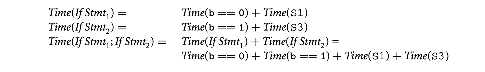
We now consider the execution time for the two possible inputs and take their maximum. Let us now consider the program for input b = 0. Since statements S1 and S4 are executed, we have:

Similarly, S2 and S3 are executed for b = 1. Thus,

The execution time estimate is set to the maximum of $\text{Time}(\text{If}{\text{Stmt}}_1;\text{If}{\text{Stmt}}_2{)}_{\text{b=0}}$ and $\text{Time}(\text{If}{\text{Stmt}}_1;\text{If}{\text{Stmt}}_2{)}_{\text{b=1}}$. Both of these quantities are lower than the estimate computed by using the default timing schema rules. Thus, by taking the maximum of these two quantities we will get a tighter estimate than by applying the vanilla timing schema rules.

Partitioning the program inputs and obtaining the WCET for each input partition is a very simple, yet powerful, idea. Even though it has been employed for execution time analysis and energy optimization in the context of timing schema [24, 25], we can plug this idea into other WCET calculation methods as well. The practical difficulty in employing this idea is, of course, computing the input partitions in general. In particular, Gheorghita et al. [25] mention the suitability of the input partitioning approach for multimedia applications performing video and audio decoding and encoding; in these applications there are different computations for different types of input frames being decoded and encoded. However, in general, it is difficult to partition the input space of a program so that inputs with similar execution time estimates get grouped to the same partition. As an example, consider the insertion sort program where the input space consists of the different possible ordering of the input elements in the input array. Thus, in an $n$-element input array, the input space consists of the different possible permutations of the array element (the permutation $a[1],a[3],a[2]$ denoting the ordering $a[1]<a[3]<a[2]$). First, getting such a partitioning will involve an expensive symbolic execution of the sorting program. Furthermore, even after we obtain the partitioning we still have too many input partitions to work with (the number of partitions for the sorting program is the number of permutations, that is, $n!$). In the worst case, each program input is in a different partition, so the WCET estimation will reduce to exhaustive simulation.

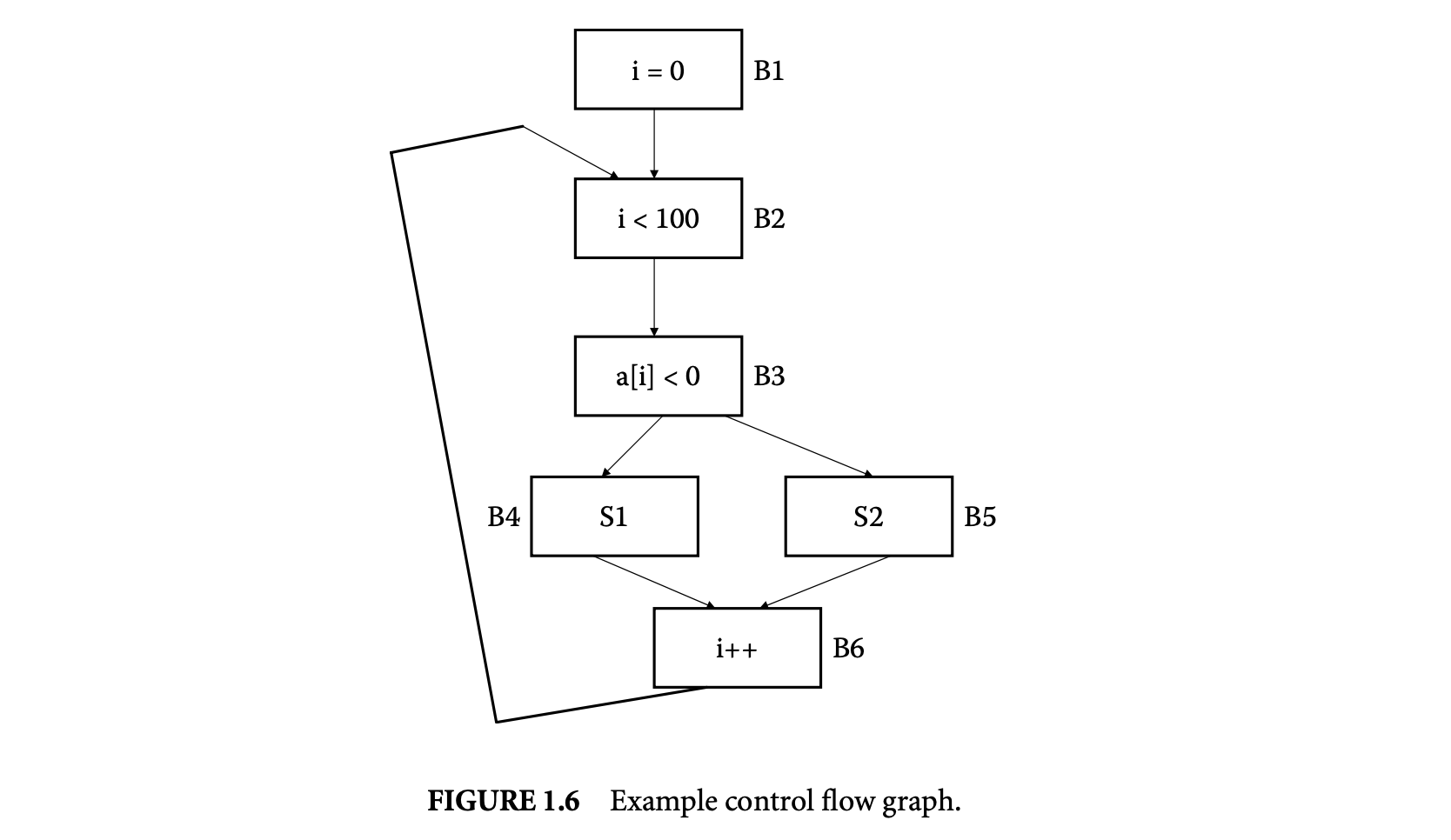
A general approach for exploiting infeasible path information in tree-based WCET calculation has been presented in [61]. In this work, the set of all paths in the control flow graph (taking into account the loop bounds) is described as a regular expression. This is always possible since the set of paths in the control flow graph (taking into account the loop bounds) is finite. Furthermore, all of the infeasible path information given by the user is also converted to regular expressions. Let Paths be the set of all paths in the control flow graph and let $I_1$, $I_2$ be certain infeasible path information (expressed as a regular expression). We can then safely describe the set of feasible paths as $\text{Paths}\cap (\neg I_1)\cap (\neg I_2)$; this is also a regular expression since regular languages are closed under negation and intersection. Timing schema now needs to be employed in these paths, which leads to a practical difficulty. To explain this point, consider the following simple program fragment.

We can draw the control flow graph of this program and present the set of paths in the control flow graph (see Figure 6) as a regular expression over basic block occurrences. Thus, the set of paths in the control flow graph fragment of Figure 6 is

Now, suppose we want to feed the information that the block B4 is executed at least in one iteration. If $a[i]$ is an input array, this information can come from our knowledge of the program input. Alternatively, if $a[i]$ was constructed via some computation prior to the loop, this information can come from our understanding of infeasible program paths. In either case, the information can be encoded as the regular expression $\neg B1(B2B3B5B6{)}^{\ast }={\Sigma }^{\ast }B4{\Sigma }^{\ast }$, where $\Sigma =\{B1,B2,B3,B4,B5,B6\}$ is the set of all basic blocks. The set of paths that the WCET analysis should consider is now given by

The timing schema approach will now remove the intersection by unrolling the loop as follows.

For each of these sets of paths (whose union we represent above) we can employ the conventional timing schema approach. However, there are 100 sets to consider because of unrolling a loop with 100 iterations. This is what makes the exploitation of infeasible paths difficult in the timing schema approach.

1.2.2.6 Exploiting Infeasible Path Information in ILP-Based WCET Calculation

Finally, we discuss how infeasible path information can be exploited in the ILP-based approach for WCET calculation. As mentioned earlier, the ILP-based approach is the most widely employed WCET calculation approach in state-of-the-art WCET estimation tools. The ILP approach reduces the WCET calculation to a problem of optimizing a linear objective function. The objective function represents the execution time of the program, which is maximized subject to flow constraints (in the control flow graph) and loop bound constraints. Note that the variables in the ILP problem correspond to execution counts of control flow graph nodes (i.e., basic blocks and edges).

Clearly, integrating infeasible path information will involve encoding knowledge of infeasible program paths as additional linear constraints [49, 68]. Introducing such constraints will make the WCET estimate (returned by the ILP solver) tighter. The description of infeasible path information as linear constraints has been discussed in several works. Park proposes an information description language (IDL) for describing infeasible path information [62]. This language provides convenient primitives for describing path information through annotations such as sampetth(A,C), where $A,C$ can be lines in the program. This essentially means than whenever $A$ is executed, $C$ is executed and vice versa (note that $A,C$ can be executed many times, as they may lie inside a loop). In terms of execution count constraints, such information can be easily encoded as $N_{B_A}=N_{B_C}$, where $B_A$ and $B_C$ are the basic blocks containing $A,C$, and $N_{B_A}$ and $N_{B_C}$ are the number of executions of $B_A$ and $B_C$.

Recent work [e.g., 20] provides a systematic way of encoding path constraints as linear constraints on execution counts of control flow graph nodes and edges. In this work, the program's behavior is described in terms of "scopes"; scope boundaries are defined by loop or function call entry and exit. Within each scope, the work provides a systematic syntax for providing path information in terms of linear constraints.

For example, let us consider the control flow graph schematic denoting two if-then-else statements within a loop shown in Figure 7. The path information is now given in terms of each/all iterations of the scope (which in this case is the only loop in Figure 7). Thus, if we want to give the information that blocks $B2$ and $B6$ are always executed together (which is equivalent to using the sampetth annotation described earlier) we can state it as $N_{B_2}=N_{B_6}$. On the other hand, if we want to give the information that B2 and B6 are never executed together (in any iteration of the loop), this gets converted to the following format

Incorporating the number of loop iterations in the above constraints, one can obtain the linear constraint $N_{B_2}+N_{B_6}\le 100$ (assuming that the loop bound is 100). This constraint is then fed to the ILP solver along with the flow constraints and loop bounds (and any other path information).

In conclusion, we note that the ILP formulation for WCET calculation relies on aggregate execution counts of basic blocks. As any infeasible path information involves sequences of basic blocks, the encoding of infeasible path information as linear constraints over aggregate execution counts can lose information (e.g., it is possible to satisfy $N_{B_2}+N_{B_6}\le 100$ in a loop with 100 iterations even if $B_2$ and $B_6$ are executed together in certain iterations). However, encoding infeasible path information as linear constraints provides a safe and effective way of ruling out a wide variety of infeasible program flows. Consequently, in most existing WCET estimation tools, ILP is the preferred method for WCET calculation.

1.3 Micro-Architectural Modeling

The execution time of a basic block $B$ in a program executing on a particular processor depends on (a) the number of instructions in $B$, (b) the execution cycles per instruction in $B$, and (c) the clock period of the processor. Let a basic block $B$ contain the sequence of instructions $⟨I_1,I_2,\dots ,I_N⟩$. For a simple micro-controller (e.g., TI MSP430), the execution latency of any instruction type is a constant. Let $latency(I_i)$ be a constant denoting the execution cycles of instruction $I_i$. Then the execution time of the basic block $B$ can be expressed as

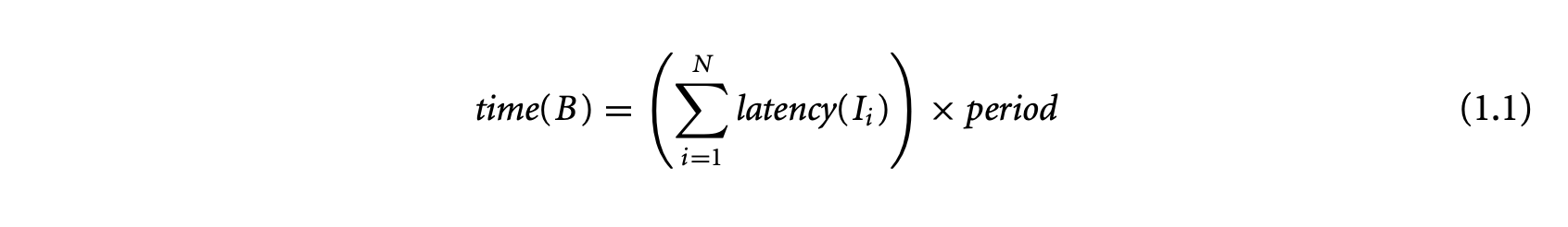
where $period$ is the clock period of the processor. Thus, for a simple micro-controller, the execution time of a basic block is also a constant and is trivial to compute. For this reason, initial work on timing analysis [67, 73] concentrated mostly on program path analysis and ignored the processor architecture.

However, the increasing computational demand of the embedded systems led to the deployment of processors with complex micro-architectural features. These processors employ aggressive pipelining, caching, branch prediction, and other features [33] at the architectural level to enhance performance. While the increasing architectural complexity significantly improves the average-case performance of an application, it leads to a high degree of timing unpredictability. The execution cycle $latency(I_i)$ of an instruction $I_i$ in Equation 1.1 is no longer a constant; instead it depends on the execution context of the instruction. For example, in the presence of a cache, the execution time of an instruction depends on whether the processor encounters a cache hit or a cache misses while fetching the instruction from the memory hierarchy. Moreover, the large difference between the cache hit and miss latency implies that assuming all memory accesses to be cache misses will lead to overly pessimistic timing estimates. Any effective estimation technique should obtain a safe but tight bound on the number of cache misses.

1.3.1 Sources of Timing Unpredictability

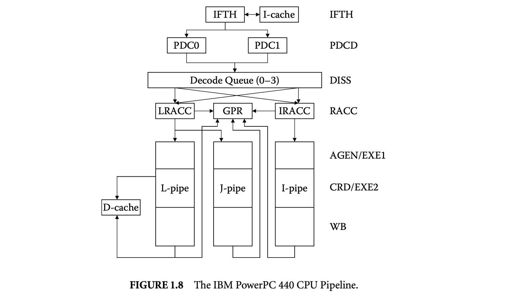
We first proceed to investigate the sources of timing unpredictability in a modern processor architecture and their implications for timing analysis. Let us use the IBM PowerPC (PPC) 440 embedded core [34] for illustration purposes. The PPC 440 is a 32-bit RISC CPU core optimized for embedded applications. It integrates a superscalar seven-stage pipeline, with support for out-of-order issue of two instructions per clock to multiple execution units, separate instruction and data caches, and dynamic branch prediction.

Figure 8 shows the PPC 440 CPU pipeline. The instruction fetch stage (IFTH) reads a cache line (two instructions) into the instruction buffer. The predecode stage (PDCD) partially decodes at most two instructions per cycle. At this stage, the processor employs a combination of static and dynamic branch prediction for conditional branches. The four-entry decode queue accepts up to two instructions per cycle from the predecode stage and completes the decoding. The decode queue always maintains the instructions in program order. An instruction waits in the decode queue until its input operands are ready and the corresponding execution pipeline is available. Up to two instructions can exit the decode queue per cycle and are issued to the register access (RACC) stage. Instruction can be issued out-of-order from the decode queue. After register access, the instructions proceed to the execution pipelines. The PPC 440 contains three execution pipelines: a load/store pipe, a simple integer pipe, and a complex integer pipe. The first execute stage (AGEN/EXE1) completes simple arithmetics and generates load/store addresses. The second execute stage (CRD/EXE2) performs data cache access and completes complex operations. The write back (WB) stage writes back the results into the register file.

Ideally, the PPC 440 pipeline has a throughput of two instructions per cycle. That is, the effective latency of each individual instruction is 0.5 clock cycle. Unfortunately, most programs encounter multiple pipeline hazards during execution that introduce bubbles in the pipeline and thereby reduce the instruction throughput:

Cache miss:: Any instruction may encounter a miss in the instruction cache (IFTH stage) and the load/store instructions may encounter a miss in the data cache (CRD/EXE2 stage). The execution of the instruction gets delayed by the cache miss latency. Data dependency:: Data dependency among the instructions may introduce pipeline bubbles. An instruction $I$ dependent on another instruction $J$ for its input operand has to wait in the decode queue until $J$ produces the result.

Control dependency:: Control transfer instructions such as conditional branches introduce control dependency in the program. Conditional branch instructions cause pipeline stalls, as the processor does not know which way to go until the branch is resolved. To avoid this delay, dynamic branch prediction in the PPC 440 core predicts the outcome of the conditional branch and then fetches and executes the instructions along the predicted path. If the prediction is correct, the execution proceeds without any delay. However, in the event of a misprediction, the pipeline is flushed and a branch misprediction penalty is incurred.

Resource contention:: The issue of an instruction from the decode queue depends on the availability of the corresponding execution pipeline. For example, if we have two consecutive load/store instructions in the decode queue, then only one of them can be issued in any cycle.

Pipeline hazards have significant impact on the timing predictability of a program. Moreover, certain functional units may have variable latency, which is input dependent. For example, the PPC 440 core can be complemented by a floating point unit (FPU) for applications that need hardware support for floating point operations [16]. In that case, the latency of an operation can be data dependent. For example, to mitigate the long latency of the floating point divide (19 cycles for single precision), the PPC 440 FPU employs an iterative algorithm that stops when the remainder is zero or the required target precision has been reached. A similar approach is employed for integer divides in some processors. In general, any unit that complies with the IEEE floating point standard [35] introduces several sources for variable latency (e.g., normalized versus denormalized numbers, exceptions, multi-path adders, etc.).

A static analyzer has to take into account the timing effect of these various architectural features to derive a safe and tight bound on the execution time. This, by itself, is a difficult problem.

1.3.2 Timing Anomaly

The analysis problem becomes even more challenging because of the interaction among the different architectural components. These interactions lead to counterintuitive timing behaviors that essentially preclude any compositional analysis technique to model the components independently.

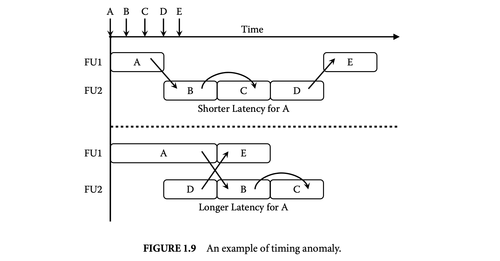
Timing anomaly is a term introduced to define the counterintuitive timing behavior [54]. Let us assume a sequence of instructions executing on an architecture starting with an initial processor state. The latency of the first instruction is modified by an amount $\Delta t$. Let $\Delta C$ be the resulting change in the total execution time of the instruction sequence.

Definition 1.2: A timing anomaly is a situation where one the following cases becomes true:

From the perspective of WCET analysis, the cases of concern are the following: (a) The (local) worst-case latency of an instruction does not correspond to the (global) WCET of the program (e.g., $\Delta t>0$ results in $\Delta C<0$), and (b) the increase in the global execution time exceeds the increase in the local instruction latency (e.g., $\Delta t>0$ results in $\Delta C>\Delta t$). Most analysis techniques implicitly assume that the worst-case latency of an instruction will lead to safe WCET estimates. For example, if the cache state is unknown, it is common to assume a cache miss for an instruction. Unfortunately, in the presence of a timing anomaly, assuming a cache miss may lead to underestimation.

1.3.2.1 Examples

An example where the local worst case does not correspond to the global worst case is illustrated in Figure 1.9. In this example, instructions A, E execute on functional unit 1 (FU1), which has variable latency. Instructions B, C, and D execute on FU2, which has a fixed latency. The arrows on the time line show when each instruction becomes ready and starts waiting for the functional unit. The processorallows out-of-order issue of the ready instructions to the functional units. The dependencies among the instructions are shown in the figure. In the first scenario, instruction A has a shorter latency, but the schedule leads to longer total execution time, as it cannot exploit any parallelism. In the second scenario, A has longer latency, preventing B from starting execution earlier (B is dependent on A). However, this delay opens up the opportunity for D to start execution earlier. This in turn allows E (which is dependent on D) to execute in parallel with B and C. The increased parallelism results in shorter overall execution time for the second scenario even though A has longer latency.

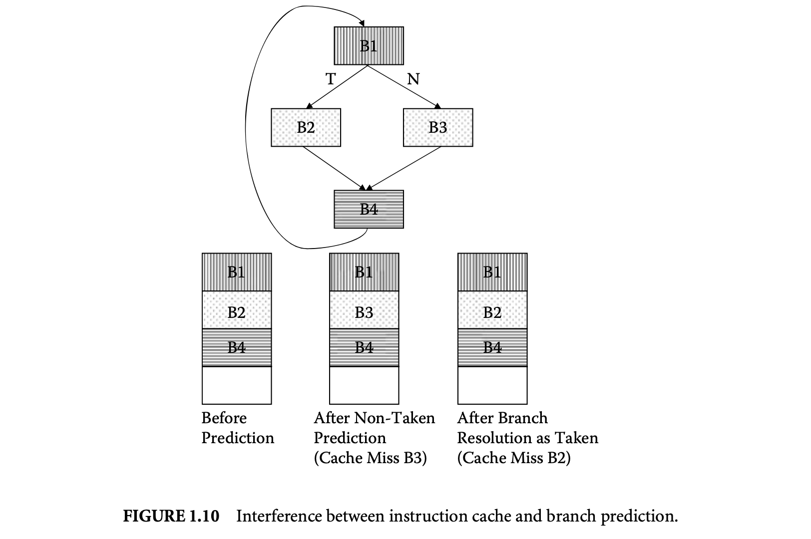
The second example illustrates that the increase in the global execution time may exceed the increase in the local instruction latency. In the PPC 440 pipeline, the branch prediction can indirectly affect instruction cache performance. As the processor caches instructions along the mispredicted path, the instruction cache content changes. This is called wrong-path instructions prefetching[63] and can have both constructive and destructive effects on the cache performance. Analyzing each feature individually fails to model this interference and therefore risks missing out on corner cases where branch misprediction introduces additional cache misses.

This is illustrated in Figure 10 with an example control flow graph. For simplicity of exposition, let us assume an instruction cache with four lines (blocks) where each basic block maps to a cache block (in reality, a basic block may get mapped to multiple cache blocks or may occupy only part of a cache block). Basic block B1 maps to the first cache block, B4 maps to the third cache block, and B2 and B3 both map to the second cache block (so they can replace each other). Suppose the execution sequence is B1 B2 B4 B1 B2 B4 B1 B2 B4... That is, the conditional branch at the end of B1 is always taken; however, it is always mispredicted. The conditional branch at the end of B4, on the other hand, is always correctly predicted. If we do not take branch prediction into account, any analysis technique will conclude a cache hit for all the basic blocks for all the iterations except for the first iteration (which encounters cold misses). Unfortunately, this may lead to underestimation in the presence of branch prediction. The cache state before the prediction at B1 is shown in Figure 10. The branch is mispredicted, leading to instruction fetch along B3. Basic block B3 incurs a cache miss and replaces B2. When the branch is resolved, however, B2 is fetched into the instruction cache after another cache miss. This will result in two additional cache misses per loop iteration. In this case, the total increase in execution time exceeds the branch misprediction penalty because of the additional cache misses. Clearly, separate analysis of instruction caches and branch prediction cannot detect these additional cache misses.

Interested readers can refer to [54] for additional examples of timing anomalies based on a simplified PPC 440 architecture. In particular, [54] presents examples where (a) a cache hit results in worst-case timing, (b) a cache miss penalty can be higher than expected, and (c) the impact of a timing anomaly on WCET may not be bounded. The third situation is the most damaging, as a small delay at the beginning of execution may contribute an arbitrarily high penalty to the overall execution time through a domino effect.

Identifying the existence and potential sources of a timing anomaly in a processor architecture remains a hard problem. Lundqvist and Stenstrom [54] claimed that no timing anomalies can occur if a processor contains only in-order resources, but Wenzel et al. [91] constructed an example of a timing anomaly in an in-order superscalar processor with multiple functional units serving an overlapping set of instruction types. A model-checking-based automated timing anomaly identification method has been proposed [18] for a simplified processor. However, the scalability of this method for complex processors is not obvious.

1.3.2.2 Implications

Timing anomalies have serious implications for static WCET analysis. First, the anomaly caused by scheduling (as shown in Figure 1.9) implies that one has to examine all possible schedules of a code fragment to estimate the longest execution time. A sequence of $n$ instructions, where each instruction can have $k$ possible latency values, generates $k^n$ schedules. Any static analysis technique that examines all possible schedules will have prohibitive computational complexity. On the other hand, most existing analysis methods rely on making safe local decisions at the instruction level and hence run the risk of underestimation.

Second, many analysis techniques adopt a compositional approach to keep the complexity of the modeling architecture under control [81, 29]. These approaches model the timing effects of the different architectural features in separation. Counterintuitive timing interference among the different features (e.g., cache and branch prediction in Figure 1.10 or cache and pipeline) may render the compositional approaches invalid. For example, Healy et al. [29] performed cache analysis followed by pipeline analysis. Whenever a memory block cannot be classified as a cache hit or miss, it is assumed to be a cache miss. This is a conservative decision in the context of cache modeling and works perfectly for the in-order processor pipeline modeled in that work. However, if it is extended to out-of-order pipeline modeling, the cache hit may instead result in worst-case timing, and the decision will not be safe.

Lundqvist and Stenstrom [54] propose a program modification method that enforces timing predictability and thereby simplifies the analysis. For example, any variable latency instruction can be preceded and succeeded by "synchronization" instructions to force serialization. Similarly, synchronization instructions and/or software-based cache prefetching can be introduced at program path merging points to ensure identical processor states, but this approach has a potentially high performance overhead and requires special hardware support.

An architectural approach to avoid complex analysis due to timing anomalies has been presented in [3]. An application is divided into multiple subtasks with checkpoints to monitor the progress. The checkpoints are inserted based on a timing analysis of a simple processor pipeline (e.g., no out-of-order execution, branch prediction, etc.). The application executes on a complex pipeline unless a subtask fails to complete before its checkpoint (which is rare). At this point, the pipeline is reconfigured to the simple mode so that the unfinished subtasks can complete in a timely fashion. However, this approach requires changes to the underlying processor micro-architecture.

1.3.3 Overview of Modeling Techniques

The micro-architectural modeling techniques can be broadly divided into two groups:

• Separated approaches
• Integrated approaches

The separated approaches work on the control flow graph, estimating the WCET of each basic block by using micro-architectural modeling. These WCET estimates are then fed to the WCET calculation method. Thus, if the WCET calculation proceeds by ILP, only the constants in the ILP problem corresponding to the WCET of the basic blocks are obtained via micro-architectural modeling.

In contrast, the integrated approaches work by augmenting a WCET calculation method with micro-architectural modeling. In the following we see at least two such examples -- an augmented ILP modeling method (to capture the timing behavior of caching and branch prediction) and an augmented timing schema approach that incorporates cache/pipeline modeling. Subsequently, we will discuss two examples of separated approaches, one of them using abstract interpretation for the micro-architectural modeling and the other one using a customized fixed-point analysis over the time intervals at which events (changing pipeline state) can occur. In both examples of the separated approach, the program path analysis proceeds by ILP.

In addition, there exist static analysis methods based on symbolic execution of the program [53]. This is an integrated method that extends cycle-accurate architectural simulation to perform symbolic execution with partially known operand values. The downside of this approach is the slow simulation speed that can lead to long analysis time.

1.3.4 Integrated Approach Based on ILP

An ILP-based path analysis technique has been described in Section 2.2. Here we present ILP-based modeling of micro-architectural components. In particular, we will focus on ILP-based instruction cache modeling proposed in [50] and dynamic branch prediction modeling proposed in [45]. We will also look at modeling the interaction between the instruction cache and the branch prediction [45] to capture the wrong-path instruction prefetching effect discussed earlier (see Figure 1.10).

The main advantage of ILP-based WCET analysis is the integration of path analysis and micro-architectural modeling. Identifying the WCET path is clearly dependent on the timing of each individual basic block, which is determined by the architectural modeling. On the other hand, behavior of instruction cache and branch prediction depends heavily on the current path. In other words, unlike pipeline, timing effects of cache and branch prediction cannot be modeled in a localized manner. ILP-based WCET analysis techniques provide an elegant solution to this problem of cyclic dependency between path analysis and architectural modeling. The obvious drawback of this method is the long solution time as the modeling complexity increases.

1.3.4.1 Instruction Cache Modeling

Caches are fast on -chip memories that are used to store frequently accessed instructions and data from main memory. Caches are managed under hardware control and are completely transparent to the programmer. Most modern processors employ separate instruction and data caches.

1.3.4.1.1 Cache Terminology

When the processor accesses an address, the address is first looked up in the cache. If the address is present in the cache, then the access is a cache hit and the content is returned to the processor. If the address is not present in the cache, then the access is a cache miss and the content is loaded from the next level of the memory hierarchy. This new content may replace some old content in the cache. The dynamic nature of the cache implies that it is difficult to statically identify cache hits and misses for an application. Indeed, this is the main problem in deploying caches in real-time systems.

The unit of transfer between different levels of memory hierarchy is called the block or line. A cache is divided into a number of sets. Let $S$ be the associativity of a cache of size $M$. Then each cache set contains $S$ cache lines. Alternatively, the cache has $S$ ways. For a direct-mapped cache, $S=1$. Further, let $B$ be the cache line size. Then the cache contains $N=\frac{M}{S\times B}$ sets. A memory block $Blk$ can be mapped to only one cache set given by (Blk\modulo\N).

1.3.4.1.2 Modeling

Li and Malik [50] first model direct-mapped instruction caches. This was later extended to set-associative instruction caches. For simplicity, we will assume a direct-mapped instruction cache here. The starting point of this modeling is again the control flow graph of the program. A basic block $B_i$ is partitioned into $n_i$ l-blocks denoted as $B_{i,1}$, $B_{i,2}$,..., $B_{i,n_i}$. A line-block, or l-block, is a sequence of code in a basic block that belongs to the same instruction cache line. Figure 1.11A shows how the basic blocks are partitioned into l-blocks. This example assumes a direct-mapped instruction cache with only two cache lines.

Let $c{m}_{i,j}$ be the total cache misses for l-block $B_{i,j}$, and $cmp$ be the constant denoting the cache miss penalty. The total execution time of the program is

where $cos{t}_i$ is the execution time of $B_i$, assuming a perfect instruction cache, and $v_i$ denotes the number of times $B_i$ is executed. This is the objective function for the ILP formulation that needs to be maximized.

The cache constraints are the linear expressions that bound the feasible values of $c{m}_{i,j}$. These constraints are generated by constructing a cache conflict graph $G_c$ for each cache line $c$. The nodes of $G_c$ are the

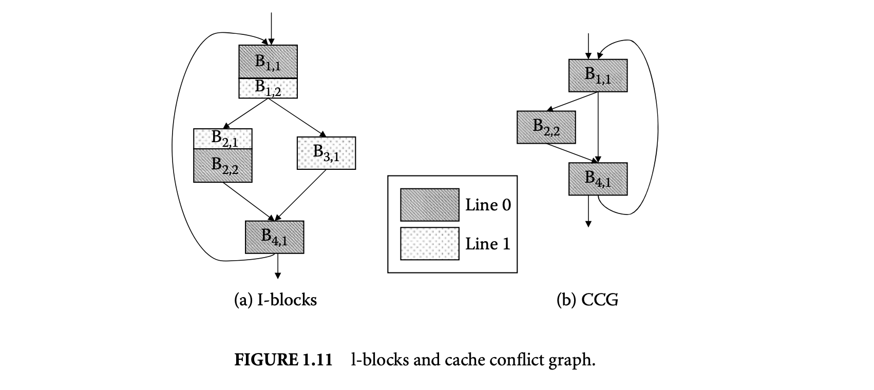
l-blocks mapped to cache line $c$. An edge $B_{i.j}\to B_{u.v}$ exists in $G_c$ if there exists a path in the control flow graph such that control flows from $B_{i.j}$ to $B_{u.v}$, without going through any other l-block mapped to $c$. In other words, there is an edge between l-blocks $B_{i.j}$ to $B_{u.v}$ if $B_{i.j}$ can be present in the cache when control reaches $B_{u.v}$. Figure 11b shows the cache conflict graph corresponding to cache line $0$ for the control flow graph in Figure 11a mapped to a cache with two lines.

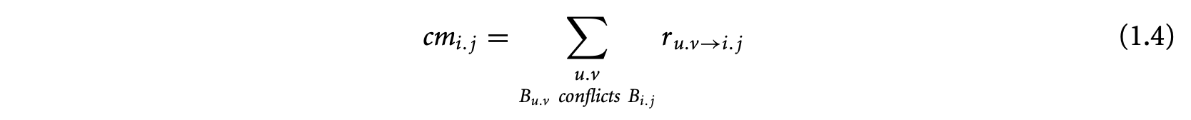
Let $r_{i.j\to u.v}$ be the execution count of the edge between l-blocks $B_{i.j}$ and $B_{u.v}$ in a cache conflict graph. Now the execution count of l-block $B_{i.j}$ equals the execution count of basic block $B_i$. Also, at each node of the cache conflict graph, the inflow equals the outflow and both equal the execution count of the node. Therefore,

The cache miss count $c{m}_{i.j}$ equals the inflow from conflicting l-blocks in the cache conflict graph. Any two1-blocks mapped to the same cache block are conflicting if they have different address tags. Two1-blocks mapped to the same cache block do not conflict when the basic block boundary is not aligned with the cache block boundary. For example, l-blocks $B_{1,2}$ and $B_{2,1}$ in Figure 11a occupy partial cache blocks and have the same address tags. They do not conflict with each other. Thus, we have

1.3.4.2 Dynamic Branch Prediction Modeling

Modern processors employ branch prediction to avoid performance loss due to control dependency [33]. Branch prediction schemes can be broadly categorized as static and dynamic. In the static scheme, a branch is predicted in the same direction every time it is executed. Though simple, static schemes are much less accurate than dynamic schemes.

1.3.4.2.1 Branch Terminology

Dynamic schemes predict a branch depending on the execution history. They use a $2^n$ entry branch prediction table to store past branch outcomes. When the processor encounters a conditional branch instruction, this prediction table is looked up using some index, and the indexed entry is used as prediction. When the branch is resolved, the entry is updated with the actual outcome. In practice, two-bit saturating counters are often used for prediction.

Different branch prediction schemes differ in how they compute an $n$-bit index to access this table. In case of simplest prediction scheme, the index is $n$ lower-order bits of the branch address. More complex schemes use a single shift register called a branch history register (BHR) to record the outcomes of the $n$ most recent branches called history $\pi$. The prediction table is looked up either using the BHR directly or exclusive or (XOR)-ed with the branch address. Considering the outcome of the neighboring branches exploits the correlation among consecutive branch outcomes.

Engblom [19] investigated the impact of dynamic branch prediction on the predicability of real-time systems. His experiments on a number of commercial processors indicate that dynamic branch prediction leads to high degree of execution time variation even for simple loops. In some cases, executing more iterations of a loop takes less time than executing fewer iterations. These results reaffirm the need to model branch prediction for WCET analysis.

1.3.4.2.2 Modeling

Li et al. [45] model dynamic branch predictors through ILP. The modeling is quite general and can be parameterized with respect to various prediction schemes. Modeling of dynamic branch prediction is somewhat similar to cache modeling. This is because they both use arrays (branch prediction table and cache) to maintain information. However, two crucial differences make branch prediction modeling significantly harder. First, a given branch instruction may use different entries of the prediction table at different points of execution (depending on the outcome of previous branches). However, an l-block always maps to the same cache block. Second, the flow of control between two conflicting l-blocks always implies a cache miss, but the flow of control between two branch instructions mapped to the same entry in the prediction table may lead to correct or incorrect prediction depending on the outcome of the two branches.

To model branch prediction, the objective function given in Equation 1.2 is modified to the following:

where $bmp$ is a constant denoting the penalty for a single branch misprediction, and $b{m}_i$ is the number of times the branch in $B_i$ is mispredicted. The constraints now need to bound feasible values of $b{m}_i$. For simplicity, let us assume that the branch prediction table is looked up using the history $\pi$ as the index.

First, a terminating least-fixed-point analysis on the control flow graph identifies the possible values of history $\pi$ for each conditional branch. The flow constraints model the change in history along the control flow graph and thereby derive the upper bound on $b{m}_i^{\pi }$ -- the execution count of the conditional branch at the end of basic block $B_i$ with history $\pi$. Next, a structure similar to a cache conflict graph is used to bound the quantity $p_{i\to j}^{\pi }$ denoting the number of times control flows from $B_i$ to $B_j$ such that the $\pi$th entry of the prediction table is used for branch prediction at $B_i$ and $B_j$ and is never accessed in between. Finally, the constraints on the number of mispredictions are derived by observing the branch outcomes for consecutive accesses to the same prediction table entry as defined by $p_{i\to j}^{\pi }$.

1.3.4.3 Interaction between Cache and Branch Prediction

Cache and branch prediction cannot be modeled individually because of the wrong-path instruction prefetching effect (see Figure 1.10). An integrated modeling of these two components through ILP to capture the interaction has been proposed in [45]. First, the objective function is modified to include the timing effect of cache misses as well as branch prediction.

If we assume that the processor allows only one unresolved branch at any time during execution, then the number of branch mispredictions $b{m}_i$ is not affected by instruction cache. However, the values of the number of cache misses $c{m}_{i,j}$ may change because of the instruction fetches along the mispredicted path. The timing effects due to these additional instruction fetches can be categorized as follows:

• An l-block $B_{i,j}$ misses during normal execution since it is displaced by another conflicting l-block $B_{u,v}$ during speculative execution (destructive effect).
• An l-block $B_{i,j}$ hits during normal execution, since it is prefetched during speculative execution (constructive effect).
• A pending cache miss of $B_{i,j}$ during speculative execution along the wrong path causes the processor to stall when the branch is resolved. How long the stall lasts depends on the portion of cache miss penalty that is masked by the branch misprediction penalty. If the speculative fetching is completely masked by the branch penalty, then there is no delay incurred.

Both the constructive and destructive effects of branch prediction on cache are modeled by modifying the cache conflict graph. The modification adds nodes to the cache conflict graph corresponding to the l-blocks fetched along the mispredicted path. Edges are added among the additional nodes as well as between the additional nodes and the normal nodes depending on the control flow during misprediction. The third factor (delay due to incomplete cache miss when the branch is resolved) is taken care of by introducing an additional delay term in Equation 1.6.

1.3.4.4 Data Cache and Pipeline

So far we have discussed instruction cache and branch prediction modeling using ILP. Data caches are harder to model than instruction caches, as the exact memory addresses accessed by load/store instructions may not be known. A simulation-based analysis technique for data caches has been proposed in [50]. A program is broken into smaller fragments where each fragment has only one execution path. For example, even though there are many possible execution paths in a JPEG decompression algorithm, the execution paths of each computational kernel such as inverse discrete cosine transform (DCT), color transformation, and so on are simple. Each code fragment can therefore be simulated to determine the number of data cache hits and misses. These numbers can be plugged into the ILP framework to estimate the WCET of the whole program. For the processor pipeline, [50] again simulates the execution of a basic block starting with an empty pipeline state. The pipeline state at the end of execution of a basic block is matched against the instructions in subsequent basic blocks to determine the additional pipeline stalls during the overlap. These pipeline stalls are added up to the execution time of the basic block. It should be obvious that this style of modeling for data cache and pipeline may lead to underestimation in the presence of a timing anomaly.

Finally, Ottosson and Sjodin [60] propose a constraint-based WCET estimation technique that extends the ILP-based modeling. This technique takes the context, that is, the history, of execution into account. Each edge in the control flow graph now corresponds to multiple variables each representing a particular program path. This allows accurate representation of the state of the cache and pipeline before a basic block is executed. A constraint-based modeling propagates the cache states across basic blocks.

1.3.5 Integrated Approach Based on Timing Schema

As mentioned in Section 2, one of the original works on software timing analysis was based on timing schema [73]. In the original work, each node of the syntax tree is associated with a simple time bound. This simple timing information is not sufficient to accurately model the timing variations due to pipeline hazards, caches, and branch prediction. The timing schema approach has been extended to model a pipeline, instruction cache, and data cache in [51].

1.3.5.1 Pipeline Modeling

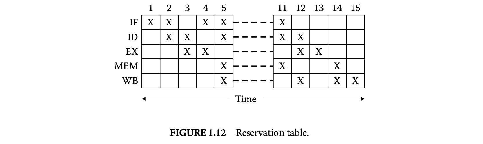
The execution time of a program construct depends on the preceding and succeeding instructions on a pipelined processor. A single time bound cannot model this timing variation. Instead a set of reservation tables associated with each program construct represents the timing information corresponding to different execution paths. A pruning strategy is used to eliminate the execution paths (and their corresponding reservation tables) that can never become the worst-case execution path of the program construct. The remaining set of reservation tables is called the worst-case timing abstraction (WCTA) of the program construct.

The reservation table represents the state of the pipeline at the beginning and end of execution of the program construct. This helps analyze the pipelined execution overlap among consecutive program constructs. The rows of the reservation table represent the pipeline stages and the columns represent time. Each entry in the reservation table specifies whether the corresponding pipeline stage is in use at the given time slot. The execution time of a reservation table is equal to its number of columns. Figure 12 shows a reservation table corresponding to a simple five-stage pipeline.

The rules corresponding to the sequence of statements and if-then-else and while-loop constructs can be extended as follows. The rule for a sequence of statements S: S1; S2 is given by

where W(S), W(S1), and W(S2) are the WCTAs of S, S1, and S2, respectively. The operator $\oplus$ is defined as

[W_{1}\oplus W_{2}={w_{1}\oplus w_{2}|w_{1}\in W_{1},w_{2}\in W_{2}}]where $w_1$ and $w_2$ are reservation tables, and $\oplus$ represents the concatenation of two reservation tables following the pipelined execution model. Similarly, the timing schema rule for S: if (exp) then S1 else S2 is given by

where $\cup$ is the set union operation. Finally, the rule for the construct S: while (exp) S1 is given by

where N is the loop bound. In all the cases, a reservation table $w$ can be eliminated from the WCTA $W$ if it can be guaranteed that w will never lead to the WCET of the program. For example, if the worst-case scenario (zero overlap with neighboring instructions) involving $w\in W$ is shorter than the best-case scenario (complete overlap with neighboring instructions) involving $w^{\prime }\in W$, then $w$ can be safely eliminated from $W$.

1.3.5.2 Instruction Cache Modeling

To model the instruction cache, the WCTA is extended to maintain the cache state information for a program construct. The main observation is that some of the memory accesses can be resolved locally (within the program construct) as cache hit/miss. Each reservation table should therefore include (a) the first reference to each cache block as its hit or miss depends on the cache content prior to the program construct (first_reference) and (b) the last reference to each cache block (last_reference). The latter affects the timing of the successor program construct(s).

The timing rules are structurally identical to the pipeline modeling, but the semantics of the $\oplus$ operator is modified. Let us assume a direct-mapped instruction cache. Then $w_1\oplus w_2$ inherits for a cache block $c$ the first_reference of $w_1$ except when $w_1$ does not have any access to $c$. In that case, $w_1\oplus w_2$ inherits the first_reference of $w_2$. Similarly, for a cache block $c$, $w_1\oplus w_2$ inherits the last_reference of $w_2$ except when $w_2$ does not have a last_reference to $c$. In this case, the last_reference to $c$ is inherited from $w_1$. Finally, the number of additional cache hits for $w_2$ can be determined by comparing the first_references of $w_2$ with the last_references of $w_1$. The execution time of $w_1\oplus w_2$ can be determined by taking into account the pipelined execution across $w_1,w_2$ and the additional cache hits. As before, a pruning strategy is employed to safely eliminate WCTA elements that can never contribute to the WCET path of the program.

1.3.5.3 Data Cache Modeling

Timing analysis of the data cache is similar to that of the instruction cache. The major difficulty, however, is that the addresses of some data references may not be known at compile time. A global data flow analysis [38] is employed to resolve the data references of load/store instructions as much as possible. A conservative approach is then proposed [38] where two cache miss penalties are assumed for each data reference whose memory address cannot be determined at compile time. The data reference is then ignored in the rest of the analysis. The first penalty accounts for the cache miss possibility of the data reference. The second penalty covers for the possibility that the data reference may replace some memory block (from the cache) that is considered as cache hit in the analysis. Finally, data dependence analysis is utilized to minimize the WCET overestimation resulting from the conservative assumption of two cache misses per unknown reference.

1.3.6 Separated Approach Based on Abstract Interpretation

ILP-based WCET analysis methods can model the architectural components and their interaction in an accurate fashion, thereby yielding tight estimates. However, ILP solution time may increase considerably with complex architectural features. To circumvent this problem, Theiling et al. [82] have proposed a separated approach where abstract interpretation is employed for micro-architectural modeling followed by ILP for path analysis. As there is a dependency between the two steps, micro-architectural modeling has to produce conservative estimates to ensure safety of the result. This overestimation is offset by significantly faster analysis time.

Abstract interpretation [15] is a theory for formally constructing conservative approximations of the semantics of a programming language. A concrete application of abstract interpretation is in static program analysis where a program's computations are performed using abstract values in place of concrete values. Abstract interpretation is used in WCET analysis to approximate the "collecting semantics" at a program point. The collecting semantics gives the set of all program states (cache, pipeline, etc.) for a given program point. In general, the collecting semantics is not computable. In abstract interpretation, the goal is to produce an abstract semantics which is less precise but effectively computable. The computation of the abstract semantics involves solving a system of recursive equations/constraints. Given a program, we can associate a variable $[[p]]$ to denote the abstract semantics at program point $p$. Clearly, $[[p]]$ will depend on the abstract semantics of program points preceding $p$. Since programs have loops, this will lead to a system of recursive constraints. The system of recursive constraints can be iteratively solved via fixed-point computation. Termination of the fixed-point computation is guaranteed only if (a) the domain of abstract values (which is used to define the abstract program semantics) is free from infinite ascending chains and (b) the iterative estimates of $[[p]]$ grow monotonically. The latter is ensured if the semantic functions in the abstract domain, which show the effect of the programming language constructs in the abstract domain and are used to iteratively estimate $[[p]]$, are monotonic.

Once the fixed-point computation terminates, for every program point $p$, we obtain a stable estimate for $[[p]]$ -- the abstract semantics at $p$. This is an overapproximation of all the concrete states with which $p$ could be reached in program executions. Thus, for cache behavior modeling, $[[p]]$ could be used to denote an overapproximation of the set of concrete cache states with which program point $p$ could be reached in program executions. This abstract semantics is then used to conservatively derive the WCET bounds for the individual basic blocks. Finally, the WCET estimates of basic blocks are combined with ILP-based path analysis to estimate the WCET of the entire program.

1.3.6.1 Cache Modeling

To illustrate AI-based cache modeling, we will assume a fully associative cache with a set of cache lines $L=\{l_1,\dots ,l_n\}$ and least recently used replacement policy. Let $\{s_1,\dots ,s_m\}$ denote the set of memory blocks. The absence of any memory block in a cache line is indicated by a new element $I$; thus, $S=\{s_1,\dots ,s_m\}\cup \{I\}$.

Let us first define the concrete semantics.

Definition 1.3: A concrete cache state is a function $c:L\to S$.

If $c(l_x)=s$ for a concrete cache state $c$, then there are $x-1$ elements $(c(l_1),\dots ,c(l_{x-1}))$ that are more recently used than $s$. In other words, $x$ is the relative age of $s$. $C_c$ denotes the set of all concrete cache states.

Definition 1.4: A cache update function $\mathcal{U}:C_c\times S\to C_c$ describes the new cache state for a given cache state and a referenced memory block.

Let $s=c(l_x)$ be the referenced memory block. The cache update function shifts the memory blocks $c(l_1),\dots ,c(l_{x-1})$, which have been more recently used than $s$, by one position to the next cache line. If $s$ was not in the cache, then all the memory blocks are shifted by one position, and the least recently used memory block is evicted from the cache state (if the cache was full). Finally, the update function puts the referenced memory block $s$ in the first position $l_1$.

The abstract semantics defines the abstract cache states, the abstract cache update function, and the join function.

Definition 1.5: An abstract cache state $\hat{c}:L\to 2^S$ maps cache lines to sets of memory blocks.

Let $\hat{C}$ denote the set of all abstract cache states. The abstract cache update function $\hat{U}:\hat{C}\times S\mapsto \hat{C}$ is a straightforward extension of the function $U$ (which works on concrete cache states) to abstract cache states.

Furthermore, at control flow merge points, join functions are used to combined the abstract cache states. That is, join functions approximate the collecting semantics depending on program analysis.

Definition 1.6: A join function $\hat{\mathcal{J}}:\hat{C}\times \hat{C}\mapsto \hat{C}$ combines two abstract cache states.

Since $L$ is finite and $S$ is finite, clearly the domain of abstract cache states is finite and hence free from any infinite ascending chains. Furthermore, the update and join functions $\hat{U}$ and $\hat{\mathcal{J}}$ are monotonic. This ensures termination of a fixed-point computation-based analysis over the above-mentioned abstract domain. We now discuss two such analysis methods.

The program analysis mainly consists of must analysis and may analysis. The must analysis determines the set of memory blocks that are always in the cache at a given program point. The may analysis determines the memory blocks that may be in the cache at a given program point. The may analysis can be used to determine the memory blocks that are guaranteed to be absent in the cache at a given program point.

The must analysis uses abstract cache states with upper bounds on the ages of the memory blocks in the concrete cache states. That is, if $s\in \hat{c}(l_x)$, then $s$ is guaranteed to be in the cache for at least the next $n-x$ memory references ($n$ is the number of cache lines). Therefore, the join function of two abstract cache states $\widehat{c_1}$ and $\widehat{c_2}$ puts a memory block $s$ in the new cache state if and only if $s$ is present in both $\widehat{c_1}$ and $\widehat{c_2}$. The new age of $s$ is the maximum of its ages in $\widehat{c_1}$ and $\widehat{c_2}$. Figure 1.13 shows an example of the join function for must and may analysis.

The may analysis uses abstract cache states with lower bounds on the ages of the memory blocks. Therefore, the join function of two abstract cache states $\widehat{c_1}$ and $\widehat{c_2}$ puts a memory block $s$ in the new cache state if $s$ is present in either $\widehat{c_1}$ or $\widehat{c_2}$ or both. The new age of $s$ is the minimum of its ages in $\widehat{c_1}$ and $\widehat{c_2}$.

At a program point, if a memory block $s$ is present in the abstract cache state after must analysis, then a memory reference to $s$ will result in a cache hit (always hit). Similarly, if a memory block $s$ is absent in the abstract cache state after may analysis, then a memory reference to $s$ will result in a cache miss (always miss). The other memory references cannot be classified as hit or miss. To improve the accuracy, a further persistence analysis can identify memory blocks for which the first reference may result in either hit or miss, but the remaining references will be hits.

These categorization of memory references is used to define the WCET for each basic block. To improve the accuracy, the WCET of a basic block is determined under different calling contexts. Thus, the objective

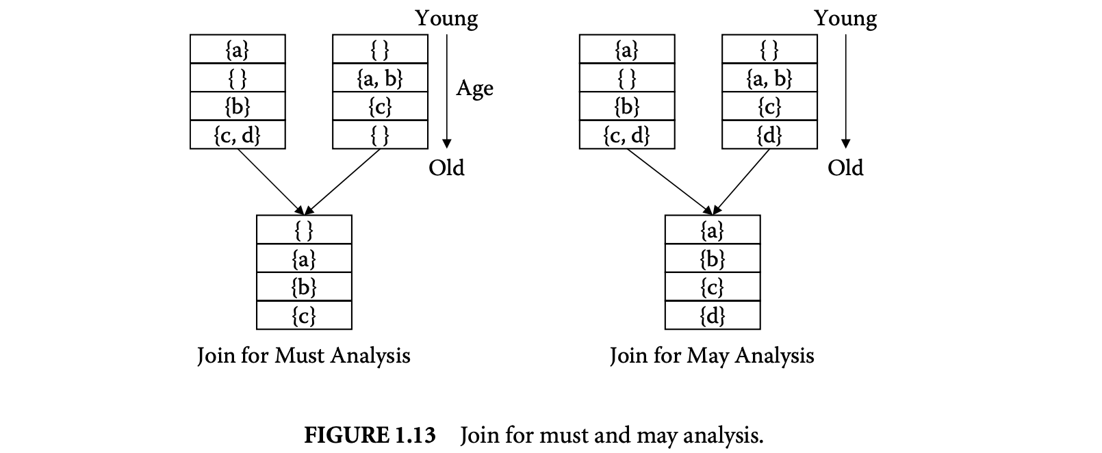
function can be defined as

where $\tau (B_i)$ denotes the set of all calling contexts for basic block $B_i$. The bounds on execution counts $v_i^x$ can be derived by ILP-based path analysis.

An extension for data cache modeling using abstract interpretation has been proposed in [23]. The basic idea is to extend the cache update function such that it can handle cases where not all addresses referenced by a basic block are known.

Another technique for categorizing cache access references into always hit, always miss, first miss, and first hit has been proposed by the group at Florida State University [4, 57, 93]. They perform categorization through static cache simulation, which is essentially an interprocedural data flow analysis. This categorization is subsequently used during pipeline analysis [29]. Pipeline analysis proceeds by determining the total number of cycles required to execute each path, where a path consists of all the instructions that can be executed during a single iteration of a loop. The data hazards and the structural hazards across paths are determined by maintaining the first and last use of each pipeline stage and register within a path. As mentioned before, this separation of cache analysis from the pipeline analysis may not be safe in the presence of a timing anomaly.

1.3.6.2 Pipeline Modeling

To model a pipeline with abstract interpretation [41], concrete execution on a concrete pipeline can be viewed as applying a function. This function takes as input a concrete pipeline state $s$ and a sequence of instructions in a basic block $b$. It produces a sequence of execution states, called a trace, and a final concrete state when executing $b$. The length of the trace determines the number of cycles the execution takes. The concept of trace is similar to the reservation table described in the context of timing-schema-based analysis.

However, in the presence of incomplete information, such as nonclassified cache accesses, the concrete execution is not feasible. Therefore, pipeline analysis employs an abstract execution of the sequence of instructions in a basic block starting with an abstract pipeline state $\hat{s}$[41]. This modeling defines an abstract pipeline state as a set of concrete pipeline states, and pipeline states with identical timing behavior are grouped together. Now, suppose that in an abstract pipeline state $\hat{s}$ an event occurs that changes the pipeline states, such as the issue/execution of an instruction $I$ in a basic block. If the latency of this event can be statically determined, $\hat{s}$ has only one successor state. However, if the latency of $I$'s execution cannot be statically determined, a pipeline state will have several successor states resulting from the execution of $I$ corresponding to the various possible latencies of $I$ (thereby causing state space explosion). In this way, reachable pipeline states within a basic block will be enumerated (while grouping together states with identical timing behavior) in order to determine the basic block's WCET.

For a processor without a timing anomaly [41], the abstract execution can be employed to each basic block starting with the empty pipeline state. The abstract execution exploits the memory reference categorization (obtained through cache modeling) to determine memory access delays during pipeline execution. Therefore, abstract execution of a basic block should happen under different contexts. In the presence of a timing anomaly, cache and pipeline analysis cannot be separated [32]. Hence the abstract states now consist of pairs of abstract pipeline states and abstract cache states. Moreover, the final abstract states of a basic block will be passed on to the successor basic block(s) as initial states. Clearly, this can lead to an exponential number of abstract states for complex processor pipelines.

1.3.6.3 Branch Prediction Modeling

Colin and Puaut [14] propose abstract-interpretation-based branch prediction modeling. They assume that the branch prediction table (see Section 1.3.4.2.1) is indexed using the address of the conditional branch instruction. This prediction scheme is simpler and hence easier to model than the BHR-based predictors modeled using ILP [45]. Colin and Puaut use the term branch target buffer (BTB) instead of prediction table, as it stores the target address in addition to the branch history. Moreover, each entry in the BTB is tagged with the address of the conditional branch instruction whose history and target address are stored in that entry. When a conditional branch is encountered, if its address is in the BTB, then it is predicted based on the history stored in the BTB. Otherwise, the default prediction of the branch not taken is used. The BTB is quite similar to instruction cache and indeed can be organized as direct-mapped or s-way set associative caches.

The abstract execution defines the abstract buffer state (ABS) corresponding to the BTB. Each basic block $B_i$ is associated with two ABS: $AB{S}_i^{in}$ and $AB{S}_i^{out}$, representing the BTB state before and after $B_i$'s execution. An ABS indicates for each BTB entry which conditional branch instructions can be in the BTB at that time. At program merge points, a set union operation is carried out. Thus,

where $\text{Pred}{B}_{(i)}$ is the set of basic blocks preceding $B_i$ in the control flow graph. Assuming a set-associative BTB, the union operator $\uplus$ is defined as follows:

where $AB{S}_i[s,k]$ is a set containing all the branch instructions that could be in the $y$th entry of the set $x$. $AB{S}_i^{out}$ is derived from $AB{S}_i^{in}$ by taking into account the conditional branch instruction in $B_i$.

Given $AB{S}_i^{in}$, the conditional branch instruction can be classified as history predicted if it is present in the BTB and default predicted otherwise. However, a history-predicted instruction does not necessarily lead to correct prediction. Similarly, a default-predicted instruction does not always lead to misprediction. This is taken into account by considering the behavior of the conditional branch instruction. For example, a history-predicted loop instruction is always correctly predicted except for loop exit.

The modeling in [14] was later extended to more complex branch predictors such as bimodal and global-history branch prediction schemes [5, 11]. The semantic context of a branch instruction in the source code is taken into account to classify a branch as easy to predict or hard to predict. Easy-to-predict branches are analyzed, while conservative misprediction penalties are assumed for hard-to-predict branches. The downside of these techniques is that they make a restrictive assumption of each branch instruction mapping to a different branch table entry (i.e., no aliasing).

1.3.7 A Separated Approach That Avoids State Enumeration

The implication of a timing anomaly (see Section 1.3.2) is that all possible schedules of instructions have to be considered to estimate the WCET of even a basic block. Moreover, all possible processor states at the end of the preceding and succeeding basic blocks have to be considered during the analysis of a basic block. This can result in state space explosion for analysis techniques, such as abstract-interpretation-based modeling, that are fairly efficient otherwise [83].

A novel modeling technique [46] obtains safe and tight estimates for processors with timing anomalies without enumerating all possible executions corresponding to variable latency instructions (owing to cache miss, branch misprediction, and variable latency functional units). In particular, [46] models a fairly complex out-of-order superscalar pipeline with instruction cache and branch prediction. First, the problem is formulated as an execution graph capturing data dependencies, resource contentions, and degree of superscalarity -- the major factors dictating instruction executions. Next, based on the execution graph, the estimation algorithm starts with very coarse yet safe timing estimates for each node of the execution graph and iteratively refines the estimates until a fixed point is reached.

1.3.7.1 Execution Graph

Figure 1.14 shows an example of an execution graph. This graph is constructed from a basic block with five instructions as shown in Figure 1.14a; we assume that the degree of superscalarity is 2. The processor has five pipeline stages: fetch (IF), decode (ID), execute (EX), write back (WB), and commit (CM). A decoded instruction is stored in the re-order buffer. It is issued (possibly out of order) to the corresponding functional unit for execution when the operands are ready and the functional unit is available.

Let $Cod{e}_B=I_1\dots I_n$ represent the sequence of instructions in a basic block $B$. Then each node $v$ in the corresponding execution graph is represented by a tuple: an instruction identifier and a pipeline stage denoted as stage(instruction_id). For example, the node $v=IF(I_i)$ represents the fetch stage of the instruction $I_i$. Each node in the execution graph is associated with the latency of the corresponding pipeline stage. For a node $u$ with variable latency $minla{t}_u\sim max$, the node is annotated with an interval $[minla{t}_u,maxla{t}_u]$. As some resources (e.g., floating point multiplier) in modern processors are fully pipelined, such resources are annotated with initiation intervals. The initiation interval of a resource is defined as the number of cycles that must elapse between issuing two instructions to that resource. For example, a fully pipelined floating point multiplier can have a latency of six clock cycles and an initiation interval of one clock cycle. For a nonpipelined resource, the initiation interval is the same as latency. Also, if there exist multiple copies of the same resource (e.g., two arithmetic logical units (ALUs)), then one needs to define the multiplicity of that resource.

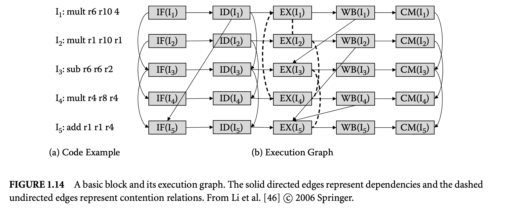
The dependence relation from node $u$ to node $v$ in the execution graph denotes that $v$ can start execution only after $u$ has completed execution; this is indicated by a solid directed edge from $u$ to $v$ in the execution graph. The analysis models the following dependencies:

• Dependencies among pipeline stages of the same instruction.
• Dependencies due to finite-sized buffers and queues such as I-buffer or ROB. For example, assuming a four-entry I-buffer, there will be no entry available for $IF(I_{i+4})$ before the completion of $ID(I_i)$ (which removes $I_i$ from the I-buffer). Therefore, there should be a dependence edge $ID(I_i)\to IF(I_{i+4})$.
• Dependencies due to in-order execution in IF, ID, and CM pipeline stages. For example, in a scalar processor (i.e., degree of $\text{superscalarity}=1$) there will be dependence edges $IF(I_i)\to IF(I_{i+1})$ because $IF(I_{i+1})$ can only start after $IF(I_i)$ completes. For a superscalar processor with $n$-way fetch (i.e., degree of $\text{superscalarity}=n$), there are dependence edges $IF(I_i)\to IF(I_{i+n})$. This captures the fact that $I_{i+n}$ cannot be fetched in the same cycle as $I_i$.
• Data dependencies among instructions. If instruction $I_i$ produces a result that is used by instruction $I_j$, then there should be a dependence edge $WB(I_i)\to EX(I_j)$.

Apart from the dependence relation among the nodes in an execution graph (denoted by solid edges), there also exist contention relations among the execution graph nodes. Contention relations model structural hazards in the pipeline. A contention relation exists between two nodes $u$ and $v$ if they can delay each other by contending for a resource, for example, functional unit or register write port. The contention between $u$ and $v$ is shown as an undirected dashed edge in the execution graph. A contention relation makes it possible for an instruction later in the program order to delay the execution of an earlier instruction.

Finally, a parallelism relation is defined to model superscalarity, for example, multiple issues and multiple decodes. Two nodes $u$ and $v$ participate in a parallelism relation iff (a) nodes $u$ and $v$ denote the same pipeline stage (call it $stg$) of two different instructions $I_i$ and $I_j$ and (b) instructions $I_i$ and $I_j$ can start execution of this pipeline stage $stg$ in parallel.

1.3.7.2 Problem Definition

Let $B$ be a basic block consisting of a sequence of instructions $Cod{e}_B=I_1\dots I_n$. Estimating the WCET of $B$ can be formulated as finding the maximum (latest) completion time of the node $CM(I_n)$, assuming that $IF(I_1)$ starts at time zero. Note that this problem is not equivalent to finding the longest path from $IF(I_1)$ to $CM(I_n)$ in $B$'s execution graph (taking the maximum latency of each pipeline stage). The execution time of a path in the execution graph is not a summation of the latencies of the individual nodes for two reasons:

• The total time spent in making the transition from $ID(I_i)$ to $EX(I_i)$ is dependent on the contentions from other ready instructions.
• The initiation time of a node is computed as the max of the completion times of its immediate predecessors in the execution graph. This models the effect of dependencies, including data dependencies.

1.3.7.3 Estimation Algorithm

The timing effects of the dependencies are accounted for by using a modified longest-path algorithm that traverses the nodes in topologically sorted order. This topological traversal ensures that when a node is visited, the completion times of all its predecessors are known. To model the effect of resource contentions, the algorithms conservatively estimate an upper bound on the delay due to contentions for a functional unit by other instructions. A single pass of the modified longest-path algorithm computes loose bounds on the lifetime of each node. These bounds are used to identify nodes with disjoint lifetimes. Thesenodes are not allowed to contend in the next pass of the longest-path search to get tighter bounds. These two steps repeat until there is no change in the bounds. Termination is guaranteed for the following reasons:

• The algorithm starts with all pairs of instructions in the contention relation (i.e., every instruction can delay every other instruction).
• At every step of the fixed-point computation, pairs are removed from this set -- those instruction pairs that are shown to be separated in time.

As the number of instructions in a basic block is finite, the number of pairs initially in the contention relation is also finite. Furthermore, the algorithm removes at least one pair in every step of the fixed-point computation, so the fixed-point computation must terminate in finitely many iterations; if the number of instructions in the basic block being estimated is $n$, the number of fixed-point iterations is bounded by $n^2$.

1.3.7.3.1 Basic Block Context

In the presence of a timing anomaly, a basic block cannot be analyzed in isolation by assuming an empty pipeline at the beginning. The instructions before (after) a basic block $B$ that directly affect the execution time of $B$ constitute the contexts of $B$ and are called the prologue (epilogue) of $B$. As processor buffer sizes are finite, the prologue and epilogue contain finite number of instructions. Of course, a basic block $B$ may have multiple prologues and epilogues corresponding to the different paths along which $B$ can be entered or exited. To capture the effects of contexts, the analysis technique constructs execution graphs corresponding to all possible combinations of prologues and epilogues. Each execution graph consists of three parts: the prologue, the basic block itself (called the body), and the epilogue.

The executions of two or more successive basic blocks have some overlap due to pipelined execution. The overlap $\delta$ between a basic block $B$ and its preceding basic block $B^{\prime }$ is the period during which instructions from both the basic blocks are in the pipeline, that is,

where $I_0$ is the last instruction of block $B^{\prime }$ (predecessor) and $I_1$ is the first instruction of block $B$. To avoid duplicating the overlap in time estimates of successive basic blocks, the execution time $t_B$ of a basic block $B$ is defined as the interval from the time when the instruction immediately preceding $B$ has finished committing to the time when $B$'s last instruction has finished committing, that is,

where $I_0$ is the instruction immediately prior to $B$ and $I_n$ is the last instruction of $B$.

The execution time for basic block $B$ is estimated with respect to (w.r.t.) the time at which the first instruction $I_1$ of $B$ is fetched, i.e., $t_{IF(I_1)}^{\text{really}}=0$. Thus, $t_B$ can be conservatively estimated by finding the largest value of $t_{CM(I_a)}^{\text{finish}}$ and the smallest value of $\delta$.

1.3.7.3.2 Overall Pipeline Analysis

The execution time estimate $t_B$ of a basic block $B$ is obtained for a specific prologue and a specific epilogue of $B$. A basic block $B$ in general has multiple choices of prologues and epilogues. Thus, $B$'s execution time is estimated under all possible combinations of prologues and epilogues. The maximum of these estimates is used as $B$'s WCET $c_B$. Let $\mathcal{P}$ and $\mathcal{E}$ be the set of prologues and epilogues for $B$.

$c_B$ is used in defining the WCET of the program as the following objective function:

The quantity $N_B$ denotes the execution count of basic block $B$ and is a variable. $\mathcal{B}$ is the set of all basic blocks in the program. This objective function is maximized over the constraints on $N_B$ given by ILP-based path analysis.

1.3.7.4 Integrating Cache and Branch Prediction Analysis

The basic idea is to define different scenarios for a basic block corresponding to cache miss and branch misprediction. If these scenarios are defined suitably, then we can estimate a constant that bounds the execution time of a basic block corresponding to each scenario. Finally, the execution frequencies of these scenarios are defined as ILP variables and are bounded by additional linear constraints.

Scenarios corresponding to cache misses are defined as follows. Given a cache configuration, a basic block $BB$ can be partitioned into a fixed number of memory blocks, with instructions in each memory block being mapped to the same cache block (cache accesses of instructions other than the first one in a memory block are always hits). A cache scenario of $BB$ is defined as a mapping of hit or miss to each of the memory blocks of $BB$. The memory blocks are categorized into always hit, always miss, or unknown, using abstract interpretation-based modeling (see Section 1.3.6.1). The upper bounds on the execution time of $BB$ are computed w.r.t. each of the possible cache scenarios. For the first instructions in memory blocks with unknown categorization, the latency of the fetch stage is assumed to be $[1,penalty]$ where $penalty$ is the cache miss penalty.

Similarly, the scenarios for branch prediction are defined as the two branch outcomes (correct prediction and misprediction) corresponding to each of the predecessor basic blocks. The execution time of the basic block is estimated w.r.t. both the scenarios by adding nodes corresponding to the wrong-path instructions to the execution graph of a basic block.

Considering the possible cache scenarios and correct or wrong prediction of the preceding branch for a basic block, the ILP objective function denoting a program's WCET is now written as follows.

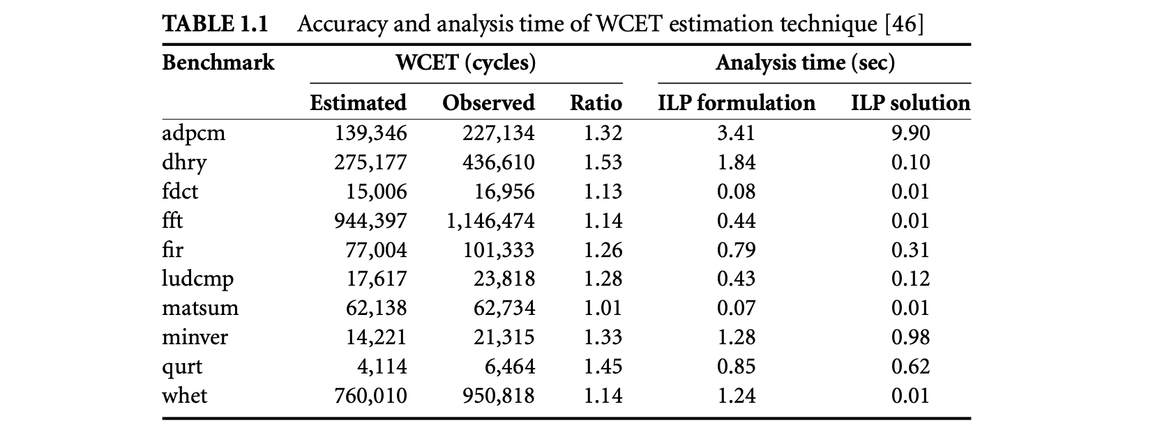
where $t_{j\to i}^{c,\omega }$ is the WCET of $B_i$ executed under the following context: (a) $B_i$ is reached from a preceding block $B_j$, (b) the branch prediction at the end of $B_j$ is correct or $B_j$ does not have a conditional branch, and (c) $B_i$ is executed under a cache scenario $\omega \in {\Omega }_i$. ${\Omega }_i$ is the set of all cache scenarios of block $B_i$. The bounds on number of scenarios with correct and mispredicted branch instructions are obtained using ILP-based analysis [45] (see Section 1.3.4.2).

Finally, to extend the above approach for modeling data caches, one can adapt the approach of [69]. This work augments the cache miss equation framework of Ghosh et al. [26] to generate accurate hit and miss patterns corresponding to memory references at different loop levels.

1.3.7.5 Accuracy and Scalability

To give the readers a feel of the accuracy and scalability of the WCET analysis techniques, we present in Table 1.1 the experimental results from [46]. The processor configuration used here is fairly sophisticated: a 2-way superscalar out-of-order pipeline with 5 stages containing a 4-entry instruction fetch buffer, an 8-entry re-order buffer, 2 ALUs, variable latency multiplication and floating point units, and 1 load/store unit; perfect data cache; gshare branch predictor with a 128-entry branch history table; a 1-KB 2-way set associative instruction cache with 16 sets, 32 bytes line size, and 30 cycles cache miss penalty. The analysis was run on a 3-GHz Pentium IV PC with 2 GB main memory.

Table 1.1 presents the estimated WCET obtained through static analysis and the observed WCET obtained via simulation (see Figure 1.3 for the terminology). The estimated WCET is quite close to the observed WCET. Also, the total estimation time (ILP formulation + ILP solving) is less than 15 seconds for all the benchmarks.

1.4 Worst-Case Energy Estimation

In this section, we present a static analysis technique to estimate safe and tight bounds for the worst-case energy consumption of a program on a particular processor. The presentation in this section is based on [36].

Traditional power simulators, such as Wattch [9] and SimplePower [96], perform cycle-by-cycle power estimation and then add them up to obtain total energy consumption. Clearly, we cannot use cycle-accurate estimation to compute the worst-case energy bound, as it would essentially require us to simulate all possible scenarios (which is too expensive). The other method [75, 88] is to use fixed per-instruction energy but it fails to capture the effects of cache miss and branch prediction. Instead, worst-case energy analysis is based on the key observation that the energy consumption of a program can be separated out into the following time-dependent and time-independent components:

Instruction-specific energy: The energy that can be attributed to a particular instruction (e.g., energy consumed as a result of the execution of the instruction in the ALU, cache miss, etc.). Instruction-specific energy does not have any relation with the execution time. Pipeline-specific energy: The energy consumed in the various hardware components (clock network power, leakage power, switch-off power, etc.) that cannot be attributed to any particular instruction. Pipeline-specific energy is roughly proportional to the execution time.

Thus, cycle-accurate simulation is avoided by estimating the two energy components separately. Pipeline-specific energy estimation can exploit the knowledge of WCET. However, switch-off power and clock network power make the energy analysis much more involved -- we cannot simply multiply the WCET by a constant power factor. Moreover, cache misses and overlap among basic blocks due to pipelining and branch prediction add significant complexity to the analysis.

1.4.1 Background

Power and energy are terms that are often used interchangeably as long as the context is clear. For battery life, however, the important metric is energy rather than power. The energy consumption of a task running on a processor is defined as $Energy=P\times t$, where $P$ is the average power and $t$ is the execution time. Energy is measured in Joules, whereas power is measured in Watts (Joules/second). Power consumption consists of two main components: dynamic power and leakage power $P=P_{dynamic}+P_{leakage}$.

Dynamic power is caused by the charging and discharging of the capacitive load on each gate's output due to switching activity. It is defined as $P_{dynamic}=\frac{1}{2}A{V}_{dd}^{2}Cf$, where $A$ is the switching activity, $V_{dd}$ is the supply voltage, $C$ is the capacitance, and $f$ is the clock frequency. For a given processor architecture, $V_{dd}$ and $f$ are constants. The capacitance value for each component of the processor can be derived through register-capacitor (RC)-equivalent circuit modeling [9].

Switching activity $A$ is dependent on the particular program being executed. For circuits that charge and discharge every cycle, such as double-ended array bitlines, an activity factor of 1.0 can be used. However, for other circuits (e.g., single-ended bitlines, internal cells of decoders, pipeline latches, etc.), an accurate estimation of the activity factor requires examination of the actual data values. It is difficult, if not impossible, to estimate the activity factors through static analysis. Therefore, an activity factor of 1.0 (i.e., maximum switching) is assumed conservatively for each active processor component.

Modern processors employ clock gating to save power. This involves switching off clock signals to the idle components so they do not consume dynamic power in the unused cycles. Jayaseelan et al. [36] model three different clock gating styles. For simplicity, let us assume a realistic gating style where idle units and ports dissipate 10% of the peak power. A multi-ported structure consumes power proportional to the number of ports accessed in a given cycle. The power consumed in the idle cycles is referred to as switch-off power.

A clock distribution network consumes a significant fraction of the total energy. Without clock gating, clock power is independent of the characteristics of the applications. However, clock gating results in power savings in the clock distribution network. Whenever the components in a portion of the chip are idle, the clock network in that portion of the chip can be disabled, reducing clock power.

Leakage power captures the power lost from the leakage current irrespective of switching activity. The analysis uses the leakage power model proposed in [98]: $P_{leakage}=V_{dd}\times N\times k_d\times I_{leakage}$, where $V_{dd}$ is the supply voltage and $N$ is the number of transistors. $I_{leakage}$ is a constant specifying the leakage current corresponding to a particular process technology. $k_d$ is an empirically determined design parameter obtained through SPICE simulation corresponding to a particular device.

1.4.2 Analysis Technique

The starting point of the analysis is the control flow graph of the program. The first step of the analysis estimates an upper bound on the energy consumption of each basic block. Once these bounds are known, the worst-case energy of the entire program can be estimated through path analysis.

1.4.2.1 Energy Estimation for a Basic Block

The goal here is to estimate a tight upper bound on the total energy consumption $energ{y}_{\text{BB}}$ of a basic block $BB$ through static analysis. From the discussion in Section 1.4.1,

where $dynami{c}_{\text{BB}}$ is the instruction-specific energy component, that is, the energy consumed as a result of switching activity as an instruction goes through the pipeline stages. $switchof{f}_{\text{BB}}$, $leakag{e}_{\text{BB}}$, and $cloc{k}_{\text{BB}}$ are defined as the energy consumed as a result of the switch-off power, leakage power, and clock power, respectively, during $wce{t}_{\text{BB}}$, where $wce{t}_{\text{BB}}$ is the WCET of the basic block $BB$. The WCET ($wce{t}_{\text{BB}}$) is estimated using the static analysis techniques. Now we describe how to define bounds for each energy component.

Dynamic EnergyThe instruction-specific energy of a basic block is the dynamic power consumed as a result of the switching activity generated by the instructions in that basic block.

where $dynami{c}_{\text{instr}}$ is the dynamic power consumed by an instruction $instr$. Now, let us analyze the energy consumed by an instruction as it travels through the pipeline:

1. Fetch and decode: The energy consumed here is due to fetch, decode, and instruction cache access. This stage needs feedback from cache analysis.
2. Register access: The energy consumed for the register file access because of reads/writes can vary from one class of instructions to another. The energy consumption in the register file for an instruction is proportional to the number of register operands.
3. Branch prediction: The energy consumption in this stage needs feedback from branch prediction modeling.
4. Wakeup logic: When an operation produces a result, the wakeup logic is responsible for making the dependent instructions ready, and the result is written onto the result bus. An instruction places the tag of the result on the wakeup logic and the actual result on the result bus exactly once, and the corresponding energy can be easily accounted for. The energy consumed in the wakeup logic is proportional to the number of output operands.
5. Selection logic: Selection logic is interesting from the point of view of energy consumption. The selection logic is responsible for selecting an instruction to execute from a pool of ready instructions. Unlike the other components discussed earlier, an instruction may access the selection logic more than once. This is because an instruction can request a specific functional unit and the request might not be granted, in which case it makes a request in the next cycle. However, we cannot accurately determine the number of times an instruction would access the selection logic. Therefore, it is conservatively assumed that the selection logic is accessed every cycle.
6. Functional units: The energy consumed by an instruction in the execution stage depends on the functional unit it uses and its latency. For variable latency instructions, one can safely assume the maximum energy consumption. The energy consumption for load/store units depends on data cache modeling.

Now, Equation 1.13, corresponding to dynamic energy consumed in a basic block $BB$, is redefined as

where ${\text{selection\_power}}_{\text{cycle}}$ is a constant defining the power consumed in the selection logic per cycle. ${\text{wcet}}_{\text{BB}}$ is the WCET of BB. Note that ${\text{dynamic}}_{\text{instr}}$ is redefined as the power consumed by $\text{instr}$ in all the pipeline stages except for selection logic.

As mentioned before, pipeline-specific energy consists of three components: switch-off energy, clock energy, and leakage energy. All three energy components are influenced by the execution time of the basic block.

Switch-off Energy

The switch-off energy refers to the power consumed in an idle unit when it is disabled through clock gating. Let ${\text{access}}_{\text{BB}}(C)$ be the total number of accesses to a component $C$ by the instructions in basic block BB. Let $\text{ports}(C)$ be the maximum number of allowed accesses/ports for component $C$ per cycle. Then, switch-off energy for component $C$ in basic block BB is

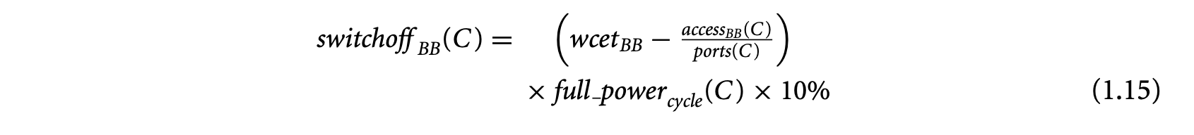
where ${\text{full\_power}}_{\text{cycle}}(C)$ is the full power consumption per cycle for component $C$. The switch-off energy corresponding to a basic block can now be defined as

where components is the set of all hardware components.

1.4.2.1.3 Clock Network Energy

To estimate the energy consumed in the clock network, clock gating should be taken into account.

where ${\text{non\_gated\_clock}}_{\text{BB}}$ is the clock energy without gating and can be defined as

where ${\text{clock\_power}}_{\text{cycle}}$ is the peak power consumed per cycle in the clock network. ${\text{circuit}}_{\text{BB}}$ is defined as the power consumed in all the components except clock network in the presence of clock gating. That is,

${\text{non\_gated\_circuit}}_{\text{BB}}$, however, is the power consumed in all the components except clock network in the absence of clock gating. It is simply defined as

${\text{circuit\_power}}_{\text{cycle}}$ is a constant defining the peak dynamic plus leakage power per cycle excluding the clock network.

1.4.2.1.4 Leakage Energy

The leakage energy is simply defined as ${\text{leakage}}_{\text{BB}}=P_{\text{leakage}}\times {\text{wcet}}_{\text{BB}}$, where $P_{\text{leakage}}$ is the power lost per processor cycle from the leakage current regardless of the circuit activity. This quantity, as defined in Section 1.4.1, is a constant given a processor architecture. ${\text{wcet}}_{\text{BB}}$ is, as usual, the WCET of BB.

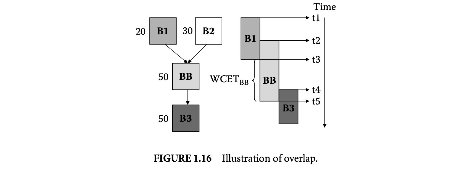
1.4.2.2 Estimation for the Whole Program

Given the energy bounds for the basic blocks, we can now estimate the worst-case energy consumption of a program using an ILP formulation. The ILP formulation is similar to the one originally proposed by Li and Malik [50] to estimate the WCET of a program. The execution times of the basic blocks are replaced with the corresponding energy consumptions. Let ${energy}_{B_i}$ be the upper bound on the energy consumption of a basic block $B_i$. Then the total energy consumption of the program is given by

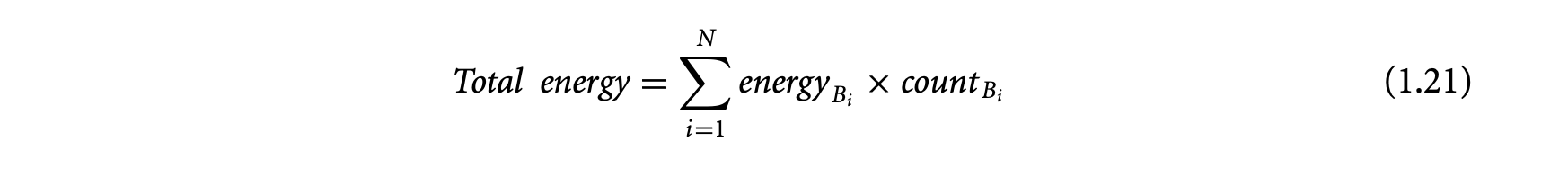
where the summation is taken over all the basic blocks in the program. The worst-case energy consumption of the program can be derived by maximizing the objective function under the flow constraints through an ILP solver.

1.4.2.3 Basic Block Context

A major difficulty in estimating the worst-case energy arises from the overlapped execution of basic blocks. Let us illustrate the problem with a simple example. Figure 1.16 shows a small portion of the control flow graph. Suppose we are interested in estimating the energy bound for basic block $BB$. The annotation for each basic block indicates the maximum execution count. This is just to show that the execution counts of overlapped basic blocks can be different. As the objective function (defined by Equation 1.21) multiplies each ${energy}_{BB}$ with its execution count ${count}_{BB}$, we cannot arbitrarily transfer energy between overlapping basic blocks. Clearly, instruction-specific energy of $BB$ should be estimated based on only the energy consumption of its instructions. However, we cannot take such a simplistic view for pipeline-specific energy. Pipeline-specific energy depends critically on ${wect}_{BB}$.

If we define ${wect}_{BB}$ without considering the overlap, that is, ${wect}_{BB}=t_5-t_2$, then it results in excessive overestimation of the pipeline-specific energy values as the time intervals $t_3-t_2$ and $t_5-t_4$ are accounted for multiple times. To avoid this, we can redefine the execution time of $BB$ as the time difference between the completion of execution of the predecessor ($B_1$ in our example) and the completion of execution of $BB$, that is, ${wect}_{BB}=t_5-t_3$. Of course, if $BB$ has multiple predecessors, then we need to estimate ${wect}_{BB}$ for each predecessor and then take the maximum value among them.

This definition of execution time, however, cannot be used to estimate the pipeline-specific energy of $BB$ in a straightforward fashion. This is because switch-off energy and thus clock network energy depend on the idle cycles for hardware ports/units. As we are looking for worst-case energy, we need to estimate an upper bound on idle cycles. Idle cycle estimation (see Equation 1.15) requires an estimate of ${access}_{BB}(C)$, which is defined as the total number of accesses to a component $C$ by the instructions in basic block $BB$. Now, with the new definition of ${wect}_{BB}$ as the interval $t_5-t_3$, not all these accesses fall within ${wect}_{BB}$, and we run the risk of underestimating idle cycles. To avoid this problem, ${access}_{BB}(C)$ in Equation 1.15 is replaced with ${\mathrm{access}}_{BB}^{WCE{T}_{BB}}(C)$ which is defined as the total number of accesses to a component C by the instructions in basic block BB that are guaranteed to occur within $wce{t}_{BB}$ The number of accesses according to this new definition is estimated during the WCET analysis of a basic block. The energy estimation techniques use the execution-graph-based WCET analysis technique [46] discussed in Section 1.3.7. Let $t_3$ be the latest commit time of the last instruction of the predecessor node $B_1$ and $let{t}_5$ be the earliest commit time of the last instruction of B B. Then, for each pipeline stage of the different instructions in B B, the algorithm checks whether its earliest or latest start time falls within the interval $t_5-t_3$. If the answer is yes, then the accesses corresponding to that pipeline stage are guaranteed to occur within $wce{t}_{BB}$ and are included in ${\mathrm{access}}_{BB}^{WCE{T}_{BB}}(C)$. The pipeline-specific energy is now estimated w.r.t. each of B B 's predecessors, and the maximum value is taken.

1.4.2.4 Integrating Cache and Branch Prediction Analysis

Integration of cache and branch prediction modeling is similar to the method described in the context of execution-graph-based WCET analysis (Section 1.3.7). For each cache scenario, the analysis adds the dynamic energy due to cache misses defined as

where $memenerg{y}_{BB}^{\omega }$ is the main memory energy for BB corresponding to cache scenario $\omega$, $miss{\omega }_{BB}^{\omega }$ is the number of cache misses in BB corresponding to cache scenario $\omega$, and $access$energy is a constant defining the energy consumption per main memory access.

The additional instruction-specific energy due to the execution of speculative instructions is estimated as follows. Let $BB$ be a basic block with $B{B}^{\prime }$ as the predecessor (see Figure 1.17). If there is a misprediction for the control flow $B{B}^{\prime }\to BB$, then instructions along the basic block B X will be fetched and executed. The executions along this mispredicted path will continue till the commit of the branch in $B{B}^{\prime }$. Let $t_3$ be the latest commit time of the mispredicted branch in $B{B}^{\prime }$. For each of the pipeline stages of the instructions along the mispredicted path (i.e., $BX$ ), the algorithm checks if its earliest start time is before $t_3$. If the answer is yes, then the dynamic energy for that pipeline stage is added to the branch misprediction energy of $BB$. In this fashion, the worst-case energy of a basic block $BB$ corresponding to all possible scenarios can be estimated, where a scenario consists of a preceding basic block $B{B}^{\prime }$ and correct/wrong prediction of the conditional branch in $B{B}^{\prime }$ and the cache scenario of $BB$.

1.4.3 Accuracy and Scalability

To give the readers a feel of the accuracy and scalability of the worst-case energy estimation technique, we present in Table 1.2 the experimental results from [36]. The processor configuration used here is as follows: an out-of-order pipeline with five stages containing a 4-entry instruction fetch buffer, an 8-entry re-order buffer, an ALU, variable latency multiplication and floating point units, and a load/store unit; perfect data cache; a gshare branch predictor with a 16-entry branch prediction table; a 4-KB 4-way set associative instruction cache, 32 bytes line size, and a 10-cycle cache miss penalty; 600 MHz clock frequency; and a supply voltage of 2.5 V.

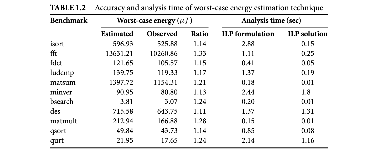
Table 1.2 presents the estimated worst-case energy obtained through static analysis and the observed worst-case energy obtained via simulation (Wattch simulator). The estimated values are quite close to the observed values. Moreover, the analysis is quite fast. It takes only $0.15\sim 2.88$ seconds to formulate the ILP problems for the benchmark programs. The ILP solver (CPLEX) is even faster and completes in under 1.8 seconds for all the benchmarks. All the experiments have been performed on a Pentium IV 1.3 GHz PC with 1 GB of memory.

1.5 Existing WCET Analysis Tools

There are some commercial and research prototype tools for WCET analysis. We discuss them in this section. The most well known and extensively used commercial WCET analyzer is the aiT tool [1] from AbsInt Angewandte Informatik. aiT takes in a code snippet in executable form and computes its WCET. The analyzer uses a two-phased approach where micro-architectural modeling is performed first followed by path analysis. It employs abstract interpretation for cache/pipeline analysis and estimates an upper bound on the execution time of each basic block. These execution time bounds of basic blocks are then combined using ILP to estimate the WCET of the entire program. Versions of aiT are available for various platforms including Motorola PowerPC, Motorola ColdFire, ARM, and so on. The aiT tool is not open-source; so the user cannot change the analyzer code to model timing effects of new processor platforms. The main strength of the aiT tool is its detailed modeling of complex micro-architectures. It is probably the only WCET estimation tool to have a full modeling of the processor micro-architecture for a complex real-life processor like Motorola ColdFire [22] and Motorola PowerPC [32].

Another commercial WCET analyzer is the Bound-T tool [87], which also takes in binary executable programs. It concentrates mainly on program path analysis and does not model cache, complex pipeline, or branch prediction. In path analysis, an important focus of the tool is inferring loop bounds, for which it extensively uses the well-known Omega-calculator [66]. Bound-T has been targeted toward Intel 8051 series micro-controllers, Analog Devices ADSP-21020 DSP, and ATMEL ERC32 SPARC V7-based platforms. Like aiT, Bound-T is not open-source.

The Chronos WCET analyzer [44] incorporates timing models of different micro-architectural features present in modern processors. In particular, it models both in-order and out-of-order pipelines, instruction caches, dynamic branch prediction, and their interactions. The modeling of different architectural features is parameterizable. Chronos is a completely open-source distribution especially suited to the needs of the research community. This allows the researcher to modify and extend the tool for his or her individual needs. Current state-of-the-art WCET analyzers, such as aiT [1], are commercial tools that do not provide the source code. Unlike other WCET analyzers, Chronos is not targeted toward one or more commercial embedded processors. Instead, it is built on top of the freely available SimpleScalar simulator infrastructure. SimpleScalar is a widely popular cycle-accurate architectural simulator that allows the user

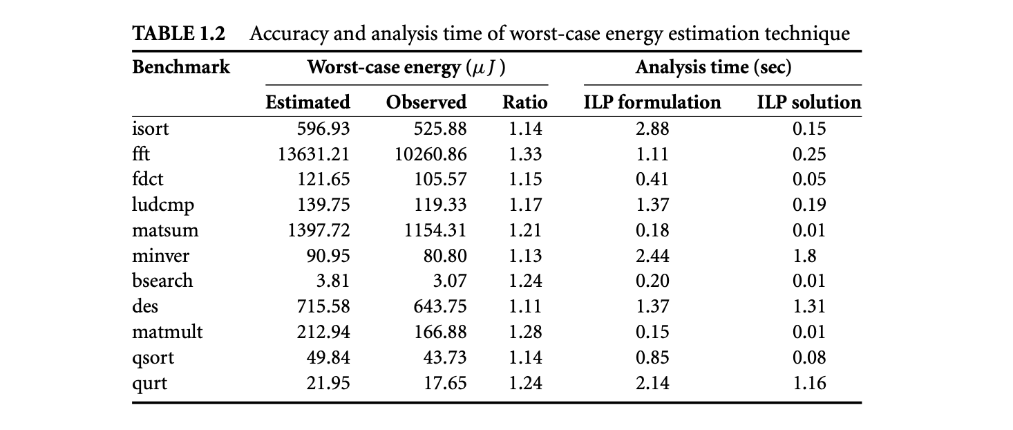
Table 1.2: Accuracy and analysis time of worst-case energy estimation technique to model a variety of processor platforms in software [10]. Chronos targets its analyzer to processor models supported by SimpleScalar. This choice of platform ensures that the user does not need to purchase a particular embedded platform and its associated compiler, debugger, and other tools (which are often fairly expensive) to conduct research in WCET analysis using Chronos. Also, the flexibility of SimpleScalar enables development and verification of modeling a variety of micro-architectural features for WCET analysis. Thus, Chronos provides a low-overhead, zero-cost, and flexible infrastructure for WCET research. However, it does not support as detailed micro-architectural modeling as is supported by the commercial aiT analyzer; in particular, certain processor features such as data cache are not modeled in Chronos.

Among the research prototypes, HEPTANE [64] is an open-source WCET analyzer. HEPTANE models in-order pipeline, instruction cache, and branch prediction, but it does not include any automated program flow analysis. Symta/P [77] is another research prototype that estimates WCET for C programs. It models caches and simple pipelines but does not support modeling of complex micro-architectural features such as out-of-order pipelines and branch prediction. Cinderella [48] is an ILP-based research prototype developed at Princeton University. The main distinguishing feature of this tool is that it performs both program path analysis and micro-architectural modeling by solving an ILP problem. However, this formulation makes the tool less scalable because the ILP solving time does not always scale up for complex micro-architectures. Also, Cinderella mostly concentrates on program path analysis and cache modeling; it does not analyze timing effects of complex pipelines and branch prediction. The SWET analyzer from Paderborn, Uppsala, and Malarden Universities focuses mostly on program flow analysis and does not model complex micro-architectures (such as out-of-order pipelines). The program flow analysis proceeds by abstract execution where variable values are abstracted to intervals. However, the abstraction in the flow analysis is limited to data values; the control flow is not abstracted. Consequently, abstract execution in the SWET tool [27] may resort to a complete unrolling of the program loops.

In addition to the above-mentioned tools, several other research groups have developed their own in-house timing analysis prototypes incorporating certain novel features. One notable effort is by the research group at Florida State University. Their work involves sophisticated flow analysis for inferring infeasible path patterns and loop bounds [31] -- features that are not commonly present in many WCET analyzers. However, the tool is currently not available for use or download; it is an in-house research effort.

1.6 Conclusions

In this chapter, we have primarily discussed software timing and energy analysis of an isolated task executing on a target processor without interruption. This is an important problem and forms the building blocks of more complicated performance analysis techniques. As we have seen, the main steps of software timing and energy analysis are (a) program path analysis and (b) micro-architectural modeling. We have also discussed a number of analysis methods that either perform an integrated analysis of the two steps or separate the two steps. It has been observed that integrated analysis methods are not scalable to large programs [94], and hence separated approaches for timing analysis may have a better chance of being integrated into compilers. Finally, we outline here some possible future research directions.

1.6.1 Integration with Schedulability Analysis

The timing and energy analysis methods discussed in this chapter assume uninterrupted execution of a program. In reality, a program (or "task," using the terminology of the real-time systems community) may get preempted because of interrupts. The major impact of task preemption is on the performance of the instruction and data caches. Let $T_l$ be a lower-priority task that gets preempted by a higher-priority task $T_h$. When $T_l$ resumes execution, some of its cache blocks have been replaced by $T_h$. Clearly, if the WCET analysis does not anticipate this preemption, the resulting timing guarantee will not be safe. Cache-related preemption delay[42, 58] analysis derives an upper bound on the number of additional cache misses per preemption. This information is integrated in the schedulability analysis [37] to derive the maximum number of possible preemptions and their effect on the worst-case cache performance.

1.6.2 System-Level Analysis

In a system-on-chip device consisting of multiple processing elements (typically on a bus), a system-wide performance analysis has to be built on top of task-level execution time analysis [70, 85]. Integrating the timing effects of shared bus and complex controllers in the WCET analysis is quite involved. In a recent work, Tanimoto et al. [80] model the shared bus on a system-on-chip device by defining bus scenario as representing a set of possible execution sequences of tasks and bus transfers. They use the definition of bus scenario to automatically derive the deadline and period for each task starting with high-level real-time requirements.

1.6.3 Retargetable WCET Analysis

Retargetability is one of the major issues that needs to be resolved for WCET analysis tools to gain wider acceptability in industry [12]. Developing a complex WCET analyzer for a new platform requires extensive manual effort. Unfortunately, the presence of a large number of platforms available for embedded software development implies that we cannot ignore this problem. The other related problem is the correctness of the abstract processor models used in static timing analysis. The manual abstraction process cannot guarantee the correctness of the models. These two problems can be solved if the static timing analyzer can be generated (semi-)automatically from a formal description of the processor.

One possibility in this direction is to start with the processor specification in some architecture description language (ADL). ADLs precisely describe the instruction-set architecture as well as the micro-architecture of a given processor platform. Certain architectural features are highly parameterizable and hence easy to retarget from a WCET analysis point of view, but other features such as out-of-order pipelines are not easily parameterizable. Li et al. [47] propose an approach to automatically generate static WCET analyzers starting from ADL descriptions for complex processor pipelines. On the other end of the spectrum, we can start with processor specification in hardware description languages (HDLs) such as Verilog or VHDL. The timing models have to be obtained from this HDL specification via simplification and abstraction. Thesing [84] takes this approach for timing models of a system controller. It remains to be seen whether this method scales to complex processor pipelines.

1.6.4 Time-Predictable System Design

The increasing complexity of systems and software leads to reduced timing predictability, which in turn creates serious difficulties for static analysis techniques [86]. An alternative is to design systems and software that are inherently more predictable in terms of timing without incurring significant performance loss. The Virtual Simple Architecture (VISA) approach [3] counters the timing anomaly problem in complex processor pipelines by augmenting the processor micro-architecture with a simpler pipeline. Proposals for predictable memory hierarchy include cache locking [89, 65], cache partitioning [95, 39], as well as replacing cache with scratchpad memory [90, 78] such that WCET analysis is simplified. At the software level, the work in [59, 28] discusses code transformations to reduce the number of program paths considered for WCET analysis. Moreover, Gustafsson et al. [28] also propose WCET-oriented programming to produce code with a very simple control structure that avoids input-data-dependent control flow decisions as far as possible.

1.6.5 WCET-Centric Compiler Optimizations

Traditional compiler optimization techniques guided by profile information focus on improving the average-case performance of a program. In contrast, the metric of importance to real-time systems is the worst-case execution time. Compiler techniques to reduce the WCET of a program have started to receive attention very recently. WCET-centric optimizations are more challenging, as the worst-case path changes as optimizations are applied.

Lee et al. [43] have developed a code generation method for dual-instruction-set ARM processors to simultaneously reduce the WCET and code size. They use a full ARM instruction set along the WCET path to achieve faster execution and at the same time we reduced Thumb instructions along the noncritical paths to reduce code size. Bodin and Puaut [8] designed a customized static branch prediction schemefor reducing a program's WCET. Zhao et al. [99] present a code positioning and transformation method to avoid the penalties associated with conditional and unconditional jumps by placing the basic blocks on WCET paths in contiguous positions whenever possible. Suhendra et al. [78] propose WCET-directed optimal and near-optimal variable allocation strategies to scratchpad memory. Finally, Yu and Mitra [97] exploit application-specific extensions to the base instruction set of a processor for reducing the WCET of real-time tasks. Clearly, there are many other contexts where WCET-guided compiler optimization can play a critical role.

Acknowledgments

Portions of this chapter were excerpted from R. Jayaseelan, T. Mitra, and X. Li, 2006, "Estimating the worst-case energy consumption of embedded software," in Proceedings of the 12th IEEE Real-Time and Embedded Technology and Applications Symposium (RTAS), pages 81-90, and adapted from X. Li, A. Roychoudhury, and T. Mitra, 2006, "Modeling out-of-order processors for WCET analysis," Real-Time Systems, 34(3): 195-227.

The authors would like to acknowledge Ramkumar Jayaseelan for preparing the figures in the introduction section.

References

[1] AbsInt Angewandte Informatik GmbH. aiT: Worst case execution time analyzer. http://www.absint.com/ait/.

[2] P. Altenbernd. 1996. On the false path problem in hard real-time programs. In Proceedings of the Eighth Euromicro Workshop on Real-Time Systems (ECRTS), 102-07.

[3] A. Anantaraman, K. Seth, K. Patil, E. Rotenberg, and F. Mueller. 2003. Virtual simple architecture (VISA): Exceeding the complexity limit in safe real-time systems. In Proceedings of the 30th IEEE/ACM International Symposium on Computer Architecture (ISCA), 350-61.

[4] R. Arnold, F. Mueller, D. B. Whalley, and M. G. Harmon. 1994. Bounding worst-case instruction cache performance. In Proceedings of the 15th IEEE Real-Time Systems Symposium (RTSS), 172-81.

[5] I. Bate and R. Reutemann. 2004. Worst-case execution time analysis for dynamic branch predictors. In Proceedings of the 16th Euromicro Conference on Real-Time Systems (ECRTS), 215-22.

[6] G. Bernat, A. Colin, and S. M. Petters. 2002. WCET analysis of probabilistic hard real-time systems. In Proceedings of the 23rd IEEE Real-Time Systems Symposium (RTSS), 279-88.

[7] R. Bodik, R. Gupta, and M. L. Soffa. 1997. Refining data flow information using infeasible paths. In Proceedings of the 6th European Software Engineering Conference held jointly with the 5th ACM SIGSOFT International Symposium on Foundations of Software Engineering ESEC/FSE, Vol. 1301 of Lecture Notes in Computer Science, 361-77. New York: Springer.

[8] F. Bodin and I. Pnuatt. 2005. A WCET-oriented static branch prediction scheme for real-time systems. In Proceedings of the 17th Euromicro Conference on Real-Time Systems, 33-40.

[9] D. Brooks, V. Tiwari, and M. Martonosi. 2000. Wattch: A framework for architectural-level power analysis and optimizations. In Proceedings of the 27th Annual ACM/IEEE International Symposium on Computer Architecture (ISCA), 83-94.

[10] D. Burger and T. Austin. 1997. The SimpleScalar tool set, version 2.0. Technical Report CS-TR-1997-1342, University of Wisconsin, Madison.

[11] C. Burguiere and C. Rochange. 2005. A contribution to branch prediction modeling in WCET analysis. In Proceedings of the IEEE Design, Automation and Test in Europe Conference and Exposition, Vol. 1, 612-17.

[12] K. Chen, S. Malik, and D. I. August. 2001. Retargetable static timing analysis for embedded software. In Proceedings of IEEE/ACM International Symposium on System Synthesis (ISSS).

[13] E. M. Clarke, E. A. Emerson, and A. P. Sistla. 1986. Automatic verification of finite-state concurrent systems using temporal logic specifications. ACM Transactions on Programming Languages and Systems 8(2):244-63.

[14] A. Colin and I. Pnuatt. 2000. Worst case execution time analysis for a processor with branch prediction. Real-Time Systems 18(2):249-74.

[15] P. Cousot and R. Cousot. 1977. Abstract interpretation: A unified lattice model for static analysis of programs by construction or approximation of fixpoints. In Proceedings of the Fourth Annual ACM Symposium on Principles of Programming Languages (POPL), 238-52.

[16] K. Dockser. 2001. "Honey, I shrunk the supercomputer!" -- The PowerPC 440 FPU brings supercomputing to IBM blue logic library. IBM MicroNews 7(4):27-29.

[17] S. Edgar and A. Burns. 2001. Statistical analysis of WCET for scheduling. In Proceedings of the 22nd IEEE Real-Time Systems Symposium (RTSS), 215-24.

[18] J. Eisinger, I. Polian, B. Becker, A. Metzner, S. Thesing, and R. Wilhelm. 2006. Automatic identification of timing anomalies for cycle-accurate worst-case execution time analysis. In Proceedings of the Ninth IEEE Workshop on Design and Diagnostics of Electronic Circuits and Systems (DDECS), 15-20.

[19] J. Engblom. 2003. Analysis of the execution time unpredictability caused by dynamic branch prediction. In Proceedings of the 9th IEEE Real-Time and Embedded Technology and Applications Symposium (RTAS), 152-59.

[20] J. Engblom and A. Ermedahl. 2000. Modeling complex flows for worst-case execution time analysis. In Proceedings of IEEE Real-Time Systems Symposium (RTSS).

[21] A. Ermedahl and J. Gustafsson. 1997. Deriving annotations for tight calculation of execution time. In Third International Euro-Par Conference on Parallel Processing (Euro-Par). Vol. 1300 of Lecture Notes in Computer Science, 1298-307. New York: Springer.

[22] C. Ferdinand, R. Heckmann, M. Langenbach, F. Martin, M. Schmidt, H. Theiling, S. Thesing, and R. Wilhelm. 2001. Reliable and precise WCET determination for a real-life processor. In Proceedings of International Workshop on Embedded Software (EMSOFT), 469-85.

[23] C. Ferdinand and R. Wilhelm. 1998. On predicting data cache behavior for real-time systems. In Proceedings of the ACM SIGPLAN Workshop on Languages, Compilers, and Tools for Embedded Systems (LCTES), 16-30.

[24] S. V. Gheorghita, T. Basten, and H. Corporaal. 2005. Intra-task scenario-aware voltage scheduling. In International Conference on Compiler, Architectures and Synthesis for Embedded Systems (CASES).

[25] S. V. Gheorghita, S. Stuijk, T. Basten, and H. Corporaal. 2005. Automatic scenario detection for improved WCET estimation. In ACM Design Automation Conference (DAC).

[26] S. Ghosh, M. Martonosi, and S. Malik. 1999. Cache miss equations: A compiler framework for analyzing and tuning memory behavior. ACM Transactions on Programming Languages and Systems, 21(4):707-46.

[27] J. Gustafsson. 2000. Eliminating annotations by automatic flow analysis of real-time programs. In Proceedings of the Seventh International Conference on Real-Time Computing Systems and Applications (RTCSA), 511-16.

[28] J. Gustafsson, B. Lisper, R. Kirner, and P. Puschner. 2006. Code analysis for temporal predictability. Real-Time Systems 32:253-77.

[29] C. Healy, R. Arnold, F. Mueller, D. Whalley, and M. Harmon. 1999. Bounding pipeline and instruction cache performance. IEEE Transactions on Computers 48(1):53-70.

[30] C. Healy, M. Sjodin, V. Rustagi, D. Whalley, and R. van Englen. 2000. Supporting timing analysis by automatic bounding of loop iterations. Real-Time Systems 18:129-56.

[31] C. A. Healy and D. B. Whalley. 2002. Automatic detection and exploitation of branch constraints for timing analysis. IEEE Transactions on Software Engineering 28(8):763-81.

[32] R. Heckmann, M. Langenbach, S. Thesing, and R. Wilhelm. 2003. The influence of processor architecture on the design and the results of WCET tools. Proceedings of the IEEE, 91(7):1038-054.

[33] J. L. Hennessy and D. A. Patterson. 2003. Computer architecture -- a quantitative approach. 3rd ed. San Francisco: Morgan Kaufmann.

[34] IBM Microelectronics Division. 1999. The PowerPC 440 core.

[35] Institute of Electrical and Electronics Engineers. 1985. IEEE 754: Standard for binary floating-point arithmetic.

[36] R. Jayaseelan, T. Mitra, and X. Li. 2006. Estimating the worst-case energy consumption of embedded software. In Proceedings of the 12th IEEE Real-Time and Embedded Technology and Applications Symposium (RTAS), 81-90.

[37] L. Ju, S. Chakraborty, and A. Roychoudhury. 2007. Accounting for cache-related preemption delay in dynamic priority schedulability analysis. In Proceedings of Design Automation and Test in Europe (DATE).

[38] S.-K. Kim, S. L. Min, and R. Ha. 1996. Efficient worst case timing analysis of data caching. In Proceedings of the Second IEEE Real-Time Technology and Applications Symposium (RTAS), 230-40.

[39] D. B. Kirk. 1989. SMART (strategic memory allocation for real-time) cache design. In Proceedings of the Real-Time Systems Symposium (RTSS), 229-39.

[40] R. Kirner. 2003. Extending optimizing compilation to support worst-case execution time analysis. PhD thesis, T. U. Vienna.

[41] M. Langenbach, S. Thesing, and R. Heckmann. Pipeline modeling for timing analysis. In Proceedings of the 9th International Symposium on Static Analysis (SAS). Vol. 2477 of Lecture Notes in Computer Science, 294-309. New York: Springer.

[42] C.-G. Lee, H. Hahn, Y.-M. Seo, S. L. Min, R. Ha, S. Hong, C. Y. Park, M. Lee, and C. S. Kim. 1998. Analysis of cache-related preemption delay in fixed-priority preemptive scheduling. IEEE Transactions on Computers 47(6):700-13.

[43] S. Lee et al. 2004. A flexible tradeoff between code size and WCET using a dual instruction set processor. In Proceedings of the 8th International Workshop on Software and Compilers for Embedded Systems (SCOPES). Vol. 3199 of Lecture Notes in Computer Science, 244-58. New York: Springer.

[44] X. Li, Y. Liang, T. Mitra, and A. Roychoudhury. Chronos: A timing analyzer for embedded software. Science of Computer Programming, special issue on Experiment Software and Toolkit 2007 (to appear), http://www.comp.nus.edu.sg/$\sim$rpembed/chronos/.

[45] X. Li, T. Mitra, and A. Roychoudhury. 2005. Modeling control speculation for timing analysis. Real-Time Systems 29(1):27-58.

[46] X. Li, A. Roychoudhury, and T. Mitra. 2006. Modeling out-of-order processors for WCET analysis. Real-Time Systems 34(3):195-227.

[47] X. Li, A. Roychoudhury, T. Mitra, P. Mishra, and X. Cheng. 2007. A retargetable software timing analyzer using architecture description language. In Proceedings of the 12th Asia and South Pacific Design Automation Conference (ASP-DAC), 396-401.

[48] Y.-T. S. Li. Cinderella 3.0 WCET analyzer. http://www.princeton.edu/$\sim$yaudil/cinderella-3.0/.

[49] Y.-T. S. Li and S. Malik. 1997. Performance analysis of embedded software using implicit path enumeration. IEEE Transactions on Computer-Aided Design of Integrated Circuits and Systems (TCAD) 16(12):1477-87.

[50] Y.-T. S. Li and S. Malik. 1998. Performance analysis of real-time embedded software. New York: Springer.

[51] S.-S. Lim, Y. H. Bae, G. T. Jang, B-D. Rhee, S. L. Min, C. Y. Park, H. Shin, K. Park, S.-M. Moon, and C. S. Kim. 1995. An accurate worst case timing analysis for RISC processors. IEEE Transactions on Software Engineering 21(7):593-604.

[52] Y. A. Liu and G. Gomez. 2001. Automatic accurate cost-bound analysis for high-level languages. IEEE Transactions on Computers 50(12):1295-309.

[53] T. Lundqvist and P. Stenstrom. 1999. An integrated path and timing analysis method based on cycle-level symbolic execution. Real-Time Systems 17(2/3):183-207.

[54] T. Lundqvist and P. Stenstrom. 1999. Timing anomalies in dynamically scheduled microprocessors. In Proceedings of the 20th IEEE Real-Time Systems Symposium (RTSS), 12-21.

[55] F. Martin, M. Alt, R. Wilhelm, and C. Ferdinand. 1998. Analysis of loops. In Compiler Construction (CC). New York: Springer.

[56] A. Metzner. 2004. Why model checking can improve WCET analysis. In Proceedings of the 16th International Conference on Computer Aided Verification (CAV). Vol. 3114 of Lecture Notes in Computer Science, 361-71. New York: Springer.

[57] F. Mueller. 2000. Timing analysis for instruction caches. Real-Time Systems 18:217-47.

[58] H. S. Negi, T. Mitra, and A. Roychoudhury. 2003. Accurate estimation of cache-related preemption delay. In Proceedings of the 1st IEEE/ACM/IFIP International Conference on Hardware/Software Codesign and System Synthesis (CODES+ISSS), 201-06.

[59] H. S. Negi, A. Roychoudhury, and T. Mitra. 2004. Simplifying WCET analysis by code transformations. In Proceedings of the 4th International Workshop on Worst-Case Execution Time Analysis (WCET).

[60] G. Ottosson and M. Sjodin. 1997. Worst-case execution time analysis for modern hardware architectures. In Proceedings of the ACM SIGPLAN Workshop on Languages, Compilers, and Tools for Real-Time Systems (LCT-RTS).

[61] C. Y. Park. 1993. Predicting program execution times by analyzing static and dynamic program paths. Real-time Systems 5(1):31-62.

[62] C. Y. Park. 1992. Predicting deterministic execution times of real-time programs. PhD thesis, University of Washington, Seattle.

[63] J. Pierce and T. Mudge. 1996. Wrong-path instruction prefetching. In Proceedings of the 29th Annual IEEE/ACM International Symposium on Microarchitectures (MICRO), 165-75.

[64] I. Pnuaut. HEPTANE static WCET analyzer. http://www.irisa.fr/aces/work/heptane-demo/heptane.html.

[65] I. Pnuaut and D. Decotigny. 2002. Low-complexity algorithms for static cache locking in multi-tasking hard real-time systems. In Proceedings of the 23rd IEEE Real-Time Systems Symposium (RTSS), 114-23.

[66] W. Pugh. 1991. The omega test: A fast and practical integer programming algorithm for dependence analysis. In ACM/IEEE Conference on Supercomputing.

[67] P. Puschner and C. Koza. 1989. Calculating the maximum execution time of real-time programs. Real-Time Systems 1(2):159-76.

[68] P. Puschner and A. Schedl. 1997. Computing maximum task execution times: A graph based approach. Real-Time Systems 13(1):67-91.

[69] H. Ramaprasad and F. Mueller. Bounding worst-case data cache behavior by analytically deriving cache reference patterns. In IEEE Real-Time Technology and Applications Symposium (RTAS), 148-57.

[70] K. Richter, D. Ziegenbein, M. Jersak, and R. Ernst. 2002. Model composition for scheduling analysis in platform design. In Proceedings of the 39th Annual ACM/IEEE Design Automation Conference (DAC), 287-92.

[71] A. Roychoudhury, T. Mitra, and H. S. Negi. 2005. Analyzing loop paths for execution time estimation. In Lecture Notes in Computer Science. Vol. 3816, 458-69. New York: Springer.

[72] T. Schuele and K. Schneider. 2004. Abstraction of assembler programs for symbolic worst case execution time analysis. In Proceedings of the 41st ACM/IEEE Design Automation Conference (DAC), 107-12.

[73] A. C. Shaw. 1989. Reasoning about time in higher-level language software. IEEE Transactions on Software Engineering 1(2):875-89.

[74] Simplify. Simplify theorem prover. http://www.research.compaq.com/SRC/esc/Simplify.html.

[75] A. Sinha and A. P. Chandrakasan. 2001. Jouletrack: A web based tool for software energy profiling. In Proceedings of the Design Automation Conference (DAC).

[76] F. Stappert, A. Ermedahl, and J. Engblom. 2001. Efficient longest executable path search for programs with complex flows and pipeline effects. In Proceedings of the First International Conference on Compilers, Architecture, and Synthesis for Embedded Systems (CASES), 132-40.

[77] J. Staschulat. Symta/P: Symbolic timing analysis for processes. http://www.ida.ing.tu-bs.de/research/projects/symta/home.e.shtml.

[78] V. Suhendra, T. Mitra, A. Roychoudhury, and T. Chen. 2005. WCET centric data allocation to scratchpad memory. In Proceedings of the 26th IEEE Real-Time Systems Symposium (RTSS), 223-32.

[79] V. Suhendra, T. Mitra, A. Roychoudhury, and T. Chen. 2006. Efficient detection and exploitation of infeasible paths for software timing analysis. In Proceedings of the 43rd ACM/IEEE Design Automation Conference (DAC), 358-63.

[80] T. Tanimoto, S. Yamaguchi, A. Nakata, and T. Higashino. 2006. A real time budgeting method for module-level-pipelined bus based system using bus scenarios. In Proceedings of the 43rd ACM/IEEE Design Automation Conference (DAC), 37-42.

[81] H. Theiling and C. Ferdinand. 1998. Combining abstract interpretation and ILP for microarchitecture modelling and program path analysis. In Proceedings of the 19th IEEE Real-Time Systems Symposium (RTSS), 144-53.

[82] H. Theiling, C. Ferdinand, and R. Wilhelm. 2000. Fast and precise WCET prediction by separated cache and path analyses. Real-Time Systems 18(2/3):157-79.

[83] S. Thesing. Safe and precise worst-case execution time prediction by abstract interpretation of pipeline models. PhD thesis, University of Saarland, Germany.

[84] S. Thesing. 2006. Modeling a system controller for timing analysis. In Proceedings of the 6th ACM/IEEE International Conference on Embedded Software (EMSOFT), 292-300.

[85] L. Thiele, S. Chakraborty, M. Gries, A. Maxiaguine, and J. Greuert. 2001. Embedded software in network processors -- models and algorithms. In Proceedings of the First International Workshop on Embedded Software (EMSOFT). Vol. 2211 of Lecture Notes in Computer Science, 416-34. New York: Springer.

[86] L. Thiele and R. Wilhelm. 2004. Design for timing predictability. Real-Time Systems, 28(2/3):157-77.

[87] Tidorum Ltd. Bound-T execution time analyzer. http://www.bound-t.com.

[88] V. Tiwari, S. Malik, and A. Wolfe. 1994. Power analysis of embedded software: A first step towards software power minimization. IEEE Transactions of VLSI Systems 2(4):437-45.

[89] X. Vera, B. Lisper, and J. Xue. 2003. Data cache locking for higher program predictability. In Proceedings of the International Conference on Measurements and Modeling of Computer Systems (SIGMETRICS), 272-82.

[90] L. Wehmeyer and P. Marwedel. 2005. Influence of memory hierarchies on predictability for time constrained embedded software. In Proceedings of the Conference on Design, Automation and Test in Europe (DATE), 600-605.

[91] I. Wenzel, R. Kirner, P. Puschner, and B. Rieder. 2005. Principles of timing anomalies in superscalar processors. In Proceedings of the Fifth International Conference on Quality Software (QSIC), 295-303.

[92] I. Wenzel, R. Kirner, B. Rieder, and P. Puschner. Measurement-based worst-case execution time analysis. In Proceedings of the Third IEEE Workshop on Software Technologies for Future Embedded and Ubiquitous Systems (SEUS), 7-10.

[93] R. White, F. Mueller, C. Healy, D. Whalley, and M. Harmon. 1997. Timing analysis for data caches and set-associative caches. In Proceedings of the Third IEEE Real-Time Technology and Applications Symposium (RTAS), 192-202.

[94] R. Wilhelm. 2004. Why AI + ILP is good for WCET, but MC is not, nor ILP alone. In Proceedings of the 5th International Conference on Verification, Model Checking, and Abstract Interpretation (VMCAI). Vol. 2937 of Lecture Notes in Computer Science, 309-22. New York: Springer.

[95] A. Wolfe. 1994. Software-based cache partitioning for real-time applications. Journal of Computer and Software Engineering, Special Issue on Hardware-Software Codesign, 2(3):315-27.

[96] W. Ye et al. 2000. The design and use of simplepower: A cycle-accurate energy estimation tool. In Proceedings of the ACM/IEEE Design Automation Conference (DAC).

[97] P. Yu and T. Mitra. 2005. Satisfying real-time constraints with custom instructions. In Proceedings of the ACM International Conference on Hardware/Software Codesign and System Synthesis (CODES+ISSS), 166-71.

[98] Y. Zhang et al. 2003. Hotleakage: A temperature-aware model of subthreshold and gate leakage for architects. Technical Report CS-2003-05, University of Virginia.

[99] W. Zhao, D. Whalley, C. Healy, and F. Mueller. 2004. WCET code positioning. In Proceedings of the 25th IEEE Real-Time Systems Symposium (RTSS), 81-91.